Transformers are RNNs: A Kernel Perspective

In this article, I will argue that transformers are RNNs. I will not merely point out formal containment; I will also explain how similar transformers and RNNs are, and what practical implications follow from that viewpoint.

Transformers are RNNs

First, I will show that transformers are RNNs.

To put it simply, a transformer is an RNN whose state is the key-value cache.

If you store the key vectors and value vectors of past tokens in an attention layer, then you can predict the next token without storing what the past tokens concretely were, or even the input text itself. Therefore, for a transformer, the key-value cache is a necessary and sufficient “state”.

Given token \( x \) as input, the transformer rule \( f(x, C) \) is applied based on the list \( C \) of key vectors and value vectors so far. This yields the next-time token \( x’ \). The key-value cache is then updated by appending the key vector and value vector computed at the current time, producing a new state \( C’ \), and the process moves to the next time step. Since the rule \( f \) itself is shared across all time steps, this computation is “recursive”.

Problems with this argument

That said, this argument is somewhat forced.

First, unlike the vector-form state of a standard RNN, \( h_t \in \mathbb{R}^d \), it uses a structured “state” \( C \) that is a list of pairs.

Second, unlike the fixed-dimensional vector \( h_t \in \mathbb{R}^d \) of a standard RNN, this “state” grows as time advances.

For purely abstract discussion these are not major issues, but in applications they create large differences in implementation and efficiency.

Below, we will see that these issues can be resolved to a considerable extent, and that transformers are RNNs even more strongly than the argument above suggests.

Review of the attention mechanism

To address these issues concretely, let us briefly review the attention mechanism.

The inputs to attention are a vector called the query \( q \in \mathbb{R}^d \), a list of vectors called keys \( c_1, c_2, \ldots, c_n \in \mathbb{R}^d \), and a list of vectors called values \( v_1, v_2, \ldots, v_n \in \mathbb{R}^m \). The output is
\[
y = \frac{\sum_{i = 1}^n \exp(\langle c_i, q \rangle) v_i}{\sum_{i = 1}^n \exp(\langle c_i, q \rangle)} \in \mathbb{R}^m.
\]
Since the denominator is only normalization, let us ignore it for now and consider the attention mechanism
\[
y = \sum_{i = 1}^n \exp(\langle c_i, q \rangle) v_i \in \mathbb{R}^m. \tag{1}
\]

Attention finds keys \( c_i \in \mathbb{R}^d \) that are similar to the query \( q \in \mathbb{R}^d \) in the sense of inner product, assigns a high weight to the corresponding values \( v_i \in \mathbb{R}^m \), and sums them.

Kernel methods

Equation (1) can be interpreted as a kernel method.

Here I assume readers who are not familiar with kernel methods, so I will introduce the basics.

Kernel methods are a general class of pattern recognition and machine learning methods based on kernel functions. A kernel function is a function \( k\colon \mathcal{X} \times \mathcal{X} \to \mathbb{R} \) that takes two data points \( x, x’ \in \mathcal{X} \) and returns a real-valued similarity.

Strictly speaking, for a similarity function to be recognized as a kernel function, it must satisfy certain conditions (such as invariance under swapping the first and second arguments). This is somewhat complex, so please refer to kernel-method textbooks for details. For this article, it is enough to recognize a kernel function as “a function that takes two data points and returns a real-valued similarity”.

The most famous kernel function is the Gaussian kernel
\[
k_G(x, x’) = \exp\left(-\frac{\|x – x’\|_2^2}{2}\right).
\]
You have likely seen the Gaussian kernel used to measure similarity in many contexts.

The core of kernel methods is the following theorem.

Theorem A function \( k\colon \mathcal{X} \times \mathcal{X} \to \mathbb{R} \) is a kernel function if and only if there exist a reproducing kernel Hilbert space \( \mathcal{H} \subset \mathbb{R}^{\mathcal{X}} \) and a function \( \phi(x)\colon \mathcal{X} \to \mathcal{H} \) such that for any \( x, x’ \in \mathcal{X} \),
\[
k(x, x’) = \langle \phi(x), \phi(x’) \rangle_{\mathcal{H}}
\]
holds.

The terminology and notation are a bit intricate, so let us organize them.

A reproducing kernel Hilbert space is a vector space satisfying certain conditions (such as having an inner product that satisfies axioms). That sounds heavy, but the important points are:

1. \( \mathcal{H} \) is a vector space, and
2. An inner product \( \langle \cdot, \cdot \rangle_{\mathcal{H}} \) is defined between elements of this vector space.

In the theorem above, \( \phi(x) \) is called a feature map. A feature map transforms data into a point (vector) in the RKHS \( \mathcal{H} \).

In words, the theorem says:

• Any kernel function can be computed in two steps: transform data with a feature map, then take an inner product.
• Conversely, a similarity computed by transforming data with a feature map and then taking an inner product is a kernel function.

This theorem applies to the Gaussian kernel as well: with a feature map \( \phi_G \), we can write
\[
k_G(x, x’) = \exp\left(-\frac{\|x – x’\|_2^2}{2}\right) = \langle \phi_G(x), \phi_G(x’) \rangle_{\mathcal{H}}.
\]

Kernel methods and attention

I will show that the similarity \( \exp(\langle c_i, q \rangle) \) appearing in attention is a kernel function.

First, by rewriting the Gaussian kernel, we obtain
\[
\begin{align}
\exp\left(-\frac{\|x – x’\|_2^2}{2}\right)
&= \exp\left(-\frac{\|x\|_2^2}{2} + \langle x, x’ \rangle – \frac{\|x’\|_2^2}{2}\right) \\
&= \exp\left(-\frac{\|x\|_2^2}{2}\right)
\exp\left(-\frac{\|x’\|_2^2}{2}\right)
\exp\left(\langle x, x’ \rangle\right). \tag{2}
\end{align}
\]
That is, the Gaussian kernel is “almost” the attention weight \( \exp(\langle x, x’ \rangle) \), differing only by a small multiplicative factor. Now consider a new feature map
\[
\phi_A(x) \stackrel{\text{def}}{=} \exp\left(\frac{\|x\|_2^2}{2}\right) \phi_G(x). \tag{3}
\]
Define a new kernel function by
\[
k_A(x, x’) \stackrel{\text{def}}{=} \langle \phi_A(x), \phi_A(x’) \rangle.
\]
Then
\[
\begin{align}
\langle \phi_A(x), \phi_A(x’) \rangle
&\stackrel{(a)}{=}
\left\langle
\exp\left(\frac{\|x\|_2^2}{2}\right) \phi_G(x),
\exp\left(\frac{\|x’\|_2^2}{2}\right) \phi_G(x’)
\right\rangle \\
&=
\exp\left(\frac{\|x\|_2^2}{2}\right)
\exp\left(\frac{\|x’\|_2^2}{2}\right)
\langle \phi_G(x), \phi_G(x’) \rangle \\
&\stackrel{(b)}{=}
\exp\left(\frac{\|x\|_2^2}{2}\right)
\exp\left(\frac{\|x’\|_2^2}{2}\right)
\exp\left(-\frac{\|x – x’\|_2^2}{2}\right) \\
&\stackrel{(c)}{=}
\exp\left(\langle x, x’ \rangle\right).
\end{align}
\]
Here, (a) follows from the definition (3) of \( \phi_A \), (b) follows from the fact that \( \phi_G \) is a feature map for the Gaussian kernel, and (c) follows from (2).

Thus, the kernel function \( k_A \) defined by the feature map \( \phi_A \) is exactly the attention weight \( \exp(\langle x, x’ \rangle) \).

Using this result, we can rewrite (1) as
\[
y = \sum_{i = 1}^n k_A(c_i, q) v_i \in \mathbb{R}^m,
\]
so attention can be interpreted as adding value vectors weighted by a kernel function.

Up to here this is merely a rephrasing. What matters is that the inner product is linear, so we can swap the order of summation and inner product. Using this, (1) can be further rewritten as
\[
\begin{align}
y
&= \sum_{i = 1}^n k_A(c_i, q) v_i \\
&= \sum_{i = 1}^n \langle \phi_A(c_i), \phi_A(q) \rangle v_i \\
&= \left\langle \sum_{i = 1}^n v_i \phi_A(c_i), \phi_A(q) \right\rangle. \tag{4}
\end{align}
\]
(If you are concerned about the type of \( v_i \phi_A(c_i) \), for the moment you can regard \( v_i \) as a scalar, or think component-wise by output dimension. One can show that this notation is valid with a careful discussion.)

Now define
\[
w_n \stackrel{\text{def}}{=} \sum_{i = 1}^n v_i \phi_A(c_i).
\]
Then (4) becomes the linear model
\[
y = \langle w_n, \phi_A(q) \rangle.
\]

Transformers are RNNs (again)

With this rewriting, the issues mentioned at the beginning are (almost) resolved.

A transformer is an RNN with state \( w_n \).

When a new token is input, the output is computed by the rule
\[
y = \langle w_n, \phi_A(q) \rangle, \tag{5}
\]
and the state is updated by the rule
\[
w_{n+1} = w_n + v_n \phi_A(c_n). \tag{6}
\]

The state-update rule is the typical RNN behavior of adding a vector to the existing state, and the output rule is also simple: an inner product between an input feature and the state.

For simplicity, we have considered only a single attention layer, but the same argument applies even when multiple attention layers are stacked or other components such as MLPs are inserted between them.

Relation to in-context learning

Expanding the state update (6), the state vector can be written as
\[
w_n = v_1 \phi_A(c_1) + v_2 \phi_A(c_2) + \ldots + v_n \phi_A(c_n). \tag{7}
\]

This means that, sequentially, the model is “learning” that when a query similar to \( \phi_A(c_i) \) arrives, it should produce an output similar to \( v_i \). As a result of this learning, we obtain the weight \( w_n \) of a linear model.

This corresponds to in-context learning. As the model processes tokens, input-output pairs are formed: for this key, the value should be this. For a new input, these pairs become evidence that determines a new output. This flow is the same as ordinary learning. The query corresponds to test data; the keys correspond to training inputs; the values correspond to training outputs. However, in in-context learning, the model parameters themselves are not changed. Learning occurs as accumulation of information into internal state rather than into parameters. A transformer “learns” the relationship between queries, keys, and values while processing tokens. In particular, if you write in the prompt “in cases like this, output like that”, that correspondence is “learned”, and in subsequent generation, outputs can be produced based on these “training data”.

In ordinary learning, namely in-weight learning, weights can similarly be written as a sum of feature maps.

Let the parameter initialization be \( \theta_0 \in \mathbb{R}^d \), and consider the kernel with feature map
\[
\phi_{\text{NT}}(x) \stackrel{\text{def}}{=} \nabla_{\theta} f(x; \theta_0) \in \mathbb{R}^d
\]
and kernel function
\[
k_{\text{NT}}(x, x’) \stackrel{\text{def}}{=} \langle \phi_{\text{NT}}(x), \phi_{\text{NT}}(x) \rangle.
\]
This kernel is called the neural tangent kernel (NTK). Data \( x, x’ \) with large similarity under this kernel can be interpreted as similar in terms of their effect on model updates, because their gradients are similar.

We train by stochastic gradient descent (SGD), updating as
\[
\theta_i = \theta_{i-1} + \alpha_i \nabla_{\theta} f(x_i; \theta_i).
\]
Here \( \alpha_i \in \mathbb{R} \) is the product of the gradient of the loss with respect to the function output, \( \frac{\partial L}{\partial f} \), and the learning rate (without loss of generality we assume the output of \( f \) is one-dimensional). The learning rate is a small positive value, and the sign of \( \frac{\partial L}{\partial f} \) depends on the loss function. If the output should be increased for that training sample, \( \alpha_i \) takes a positive value; if the output should be decreased, \( \alpha_i \) takes a negative value. Suppose training yields parameters \( \theta_n \).

Assume parameters did not move much during training, and approximate by first-order Taylor expansion around \( \theta = \theta_0 \). Then the function represented by \( \theta_n \) can be written as
\[
\begin{align}
y = f(x; \theta_n)
&\approx f(x; \theta_0) + \langle (\theta_n – \theta_0), \nabla_{\theta} f(x; \theta_0) \rangle \\
&= f(x; \theta_0) + \langle (\theta_n – \theta_0), \phi_{\text{NT}}(x) \rangle \\
&= f(x; \theta_0) + \left\langle \sum_{i = 1}^{n} (\theta_i – \theta_{i-1}), \phi_{\text{NT}}(x) \right\rangle \\
&= f(x; \theta_0) + \left\langle \sum_{i = 1}^{n} \alpha_i \nabla_{\theta} f(x_i; \theta_i), \phi_{\text{NT}}(x) \right\rangle \\
&\stackrel{\text{(a)}}{\approx}
f(x; \theta_0) + \left\langle \sum_{i = 1}^{n} \alpha_i \phi_{\text{NT}}(x_i), \phi_{\text{NT}}(x) \right\rangle \tag{8} \\
&= f(x; \theta_0) + \sum_{i = 1}^{n} \alpha_i \langle \phi_{\text{NT}}(x_i), \phi_{\text{NT}}(x) \rangle \\
&= f(x; \theta_0) + \sum_{i = 1}^{n} \alpha_i k_{\text{NT}}(x_i, x). \tag{9}
\end{align}
\]
Here, in (a) we approximated \( f(x_i; \theta_i) \approx f(x_i; \theta_0) \). For a test data point \( x \) that is not similar to any training data \( x_i \), the kernel values in the second term of (9) become zero, so the output equals the initial model output \( f(x; \theta_0) \). If the test data \( x \) is similar to some training data \( x_i \), then the term \( \alpha_i k_{\text{NT}}(x_i, x) \approx \langle (\theta_i – \theta_{i-1}), \phi_{\text{NT}}(x) \rangle \) is nonzero, and the output becomes the initial model plus the learned update \( (\theta_i – \theta_{i-1}) \) from that training data \( x_i \). If \( x \) is similar to multiple training data points, all of those learned updates are added. Recall that if the output should be increased for a training sample, \( \alpha_i \) is positive, and if the output should be decreased, \( \alpha_i \) is negative. If for a similar training sample \( x_i \) the output should be increased, then \( \alpha_i k_{\text{NT}}(x_i, x) \) is positive; if it should be decreased, then it is negative. The trained model output is the accumulation of these effects.

Also, in (8), if we define
\[
w_n \stackrel{\text{def}}{=} \alpha_1 \phi_{\text{NT}}(x_1) + \alpha_2 \phi_{\text{NT}}(x_2) \ldots + \alpha_n \phi_{\text{NT}}(x_n), \tag{10}
\]
then the output of the trained model becomes
\[
y = f(x; \theta_0) + \langle w_n, \phi_{\text{NT}}(x) \rangle.
\]

Equations (7) and (10) are very similar. Whether in-weight learning or in-context learning, learning can be viewed as the procedure of measuring similarity to past data via a kernel, and determining a new output based on what the output should be on similar past data.

To a finite dimension

The problems are mostly resolved, but the discussion so far still has a somewhat forced part.

So far, I have not described how to compute \( \phi_G \) and \( \phi_A \) concretely. They are indeed “vectors”, but they are actually infinite-dimensional “vectors”, and cannot be computed explicitly.

If they cannot be computed explicitly, it may seem that everything becomes meaningless in applications. However, this is not a major issue: with a bit of ingenuity, applications remain possible.

First, \( \phi_G \) and \( \phi_A \) can be approximated accurately by finite-dimensional feature maps. There are many methods, but the simplest is to use random features. Sample random vectors \( \omega_1, \ldots, \omega_D \sim \mathcal{N}(0, 1) \in \mathbb{R}^d \) in advance, and define the finite-dimensional feature map
\[
\begin{align}
\phi_F(x) \stackrel{\text{def}}{=}
\frac{\exp(-\frac{\|x\|_2^2}{2})}{\sqrt{2D}}
\begin{bmatrix}
\exp(\langle \omega_1, x \rangle) \\
\exp(-\langle \omega_1, x \rangle) \\
\exp(\langle \omega_2, x \rangle) \\
\exp(-\langle \omega_2, x \rangle) \\
\vdots \\
\exp(\langle \omega_D, x \rangle) \\
\exp(-\langle \omega_D, x \rangle)
\end{bmatrix}
\in \mathbb{R}^{2D}.
\end{align}
\]
Then the attention weight can be approximated as
\[
k_A(x, x’) = \exp(\langle x, x’ \rangle) \approx \langle \phi_F(x), \phi_F(x’) \rangle.
\]

For example, when \( D = 100 \) and we use a 200-dimensional feature map, the code and results are as follows.

import matplotlib.pyplot as plt
import numpy as np

d = 100  # Dimension of the input vectors
n = 1000  # Number of input samples
x = np.random.randn(n, d) / np.sqrt(d)  # Generate samples
y = np.random.randn(n, d) / np.sqrt(d)  # Generate samples
gt = np.exp((x * y).sum(axis=1))  # True inner-product weight

D = 100  # Dimension of random features
omega = np.random.randn(D, d)

rx = (
    np.exp(-(x * x).sum(axis=1, keepdims=True) / 2)
    * np.hstack([np.exp(x @ omega.T), np.exp(-x @ omega.T)])
    * np.sqrt(1 / (2 * D))
)  # Random features
ry = (
    np.exp(-(y * y).sum(axis=1, keepdims=True) / 2)
    * np.hstack([np.exp(y @ omega.T), np.exp(-y @ omega.T)])
    * np.sqrt(1 / (2 * D))
)  # Random features
rf = (rx * ry).sum(axis=1)  # Approximation via random features

for i in range(10):
    print(f'Exact value: {gt[i]:.2f}, Approx value: {rf[i]:.2f}')

plt.scatter(gt, rf)  # Plot

# Example output:
# Exact value: 1.13, Approx value: 1.35
# Exact value: 1.11, Approx value: 1.10
# Exact value: 1.04, Approx value: 0.83
# Exact value: 0.89, Approx value: 1.07
# Exact value: 1.00, Approx value: 1.06
# Exact value: 1.26, Approx value: 1.10
# Exact value: 1.06, Approx value: 1.05
# Exact value: 1.07, Approx value: 1.23
# Exact value: 1.12, Approx value: 1.10
# Exact value: 1.17, Approx value: 0.95

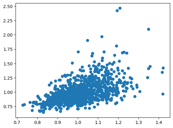
When the exact attention weight (= computed via an infinite-dimensional feature map) is 1.13, the approximation by a 100-dimensional feature map can be 1.35, for instance. This is a reasonably accurate approximation. As the dimension increases, the approximation becomes more accurate.

Therefore, if we replace every occurrence of \( \phi_A \) (infinite-dimensional) in the discussion above by \( \phi_F \) (finite-dimensional), we obtain an RNN that is computable in finite dimension.

The method above is general and simple and makes no assumptions about data properties, but when the data has good structure, one can approximate with lower dimension and higher accuracy. The idea is the same as dimension reduction by principal component analysis. Even if data is apparently 1000-dimensional, if its intrinsic dimensionality is small, one can reduce to 30 dimensions via PCA with little loss of information. That is, compression from 1000 dimensions to 30 dimensions is possible. Since an RKHS is still a vector space, something almost identical can be done there as well: compress from infinite dimension down to 30 dimensions. This makes it possible, for example, to represent a transformer as a 30-dimensional RNN. Methods that approximate feature maps based on intrinsic low dimensionality of data include the Nystrom approximation.

Second, even though \( \phi_G \) and \( \phi_A \) cannot be computed exactly, there is no reason to cling to them. The essence of attention is to add value vectors weighted by a kernel, as in
\[
y = \sum_{i = 1}^n k(c_i, q) v_i \in \mathbb{R}^m,
\]
and there is no necessity to use \( k_A \) as the kernel. Many kernels can be represented by finite-dimensional feature maps, and using such kernels removes this issue. Choosing kernels for attention that achieve both accuracy and efficiency remains an active research topic. A representative result is linear transformers such as Katharopoulos+ ICML 2020.

Application to acceleration

From the above, we have two equivalent views of transformers: the conventional transformer-mode formula (1), and the RNN-mode formulas (5, 6).

People often say “transformers are easier to train in parallel than RNNs” or “transformers require quadratic time and have larger complexity than RNNs”, but these claims are about fixing one viewpoint, and are not intrinsic properties of transformers. The same transformer model can be run in both transformer mode (1) and RNN mode (5, 6). For example, during training we can run it in transformer mode, which is easier to parallelize, and during inference we can run it in RNN mode, which uses less memory and computation. Even for the same model, flexible handling is possible.

Handling the denominator

As a minor point, we have ignored the denominator
\[
\sum_{i = 1}^n \exp(\langle c_i, q \rangle)
\]
so far. With the kernel-method viewpoint, you can see that this term can also be written as a linear model:
\[
\begin{align}
\sum_{i = 1}^n \exp(\langle c_i, q \rangle)
&= \sum_{i = 1}^n \langle \phi_A(c_i), \phi_A(q) \rangle \\
&= \left\langle \sum_{i = 1}^n \phi_A(c_i), \phi_A(q) \right\rangle \\
&= \langle u_n, \phi_A(q) \rangle.
\end{align}
\]
Therefore, the denominator can be expressed in an RNN-like way as well, and the whole numerator/denominator can be expressed similarly. Including the denominator does not change the discussion above.

Transformers are RNNs (again, again)

From the discussion above, transformers and RNNs are not a binary opposition; rather, they can be considered the same kind of thing viewed from different angles.

Quantitatively, the dimension of the state \( w_n \) has a large effect. Using the Gaussian kernel, or the exponent of an inner product as commonly used in transformers, yields an infinite-dimensional vector space. This space is extremely large, so in principle it can remember infinitely many things, but it is hard to compute efficiently, it can overfit, and it can require lots of training data. If we use other kernels or approximate in the spirit of PCA, we obtain finite dimension; as we reduce dimension, computational efficiency and sample efficiency improve. This is not a forced either-or choice, but a continuous spectrum: at one extreme is the exponent-of-inner-product kernel used in conventional transformers, and along the spectrum lie high-dimensional RNNs, medium-dimensional RNNs, and low-dimensional RNNs.

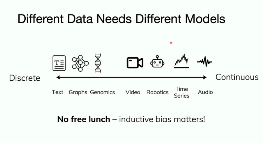
We can choose kernels and compression levels based on the nature of the data. For example, text is discrete and each token has large granularity; forgetting even a small number of tokens can cause problems in future responses. Therefore, for text, it is better to do little compression and use an infinite-dimensional state space or something close to it, as in conventional transformers, to remember the input almost as-is. In contrast, video and audio are continuous; losing some frames does not cause issues, and substantial compression is possible. In such cases, it is better to use a more RNN-like, more highly compressed, lower-dimensional state space and process while compressing. Even within the same domain, you can decide where to stand on this spectrum by considering how much compression seems possible given the distribution and task.

This relationship among “compression”, “generalization”, and “efficiency” is very important for understanding model behavior. Viewing transformers as RNNs makes the degree of compression explicit as the state dimension, which is also useful because it enables us to handle this three-way relationship consciously.

Author Profile

If you found this article useful or interesting, I would be delighted if you could share your thoughts on social media.

New posts are announced on @joisino_en (Twitter), so please be sure to follow!