A Gentle Introduction to Machine Learning Theory

When I first began learning about machine learning, I struggled with the notion that lowering the loss on the training data does not necessarily guarantee performance on the test data, since training data and test data are different.

In this article, I will carefully explain why the performance on test data is theoretically guaranteed, aiming to help beginners in statistics and machine learning — including my former self.

By the end of this article, I will extend this discussion to the theory of deep learning and connect it to cutting-edge research. The goal is to demonstrate how one can reach advanced topics solely from basic concepts such as expectation and variance. Please stay with me until the end.

Concentration around the Expectation

First, let’s discuss the phenomenon where the average of independent data concentrates around the expected value.

You might have heard of the law of large numbers. When you roll a die, 10 dice, and 100 dice, the average value approaches the expected value, \(3.5\).

Let’s actually verify this phenomenon.

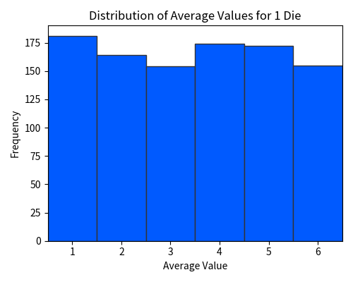
First, consider rolling a single die. In this case, naturally, each number from 1 to 6 appears with equal probability. With a sample size of 1, the average value is simply the value that comes up.

Next, let us roll 10 dice and calculate their average. Each experiment corresponds to rolling 10 dice. We repeat this process.

Now, let us visualize the average values — the final column outlined in red in the table above. The following figure plots the 1000 “averages” obtained from 1000 experiments.

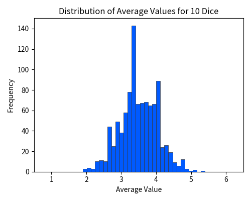
Unlike the case of a single die roll, you can see that the values here are clearly concentrated around \(3.5\).

Next, let us try rolling 100 dice.

After conducting 1000 experiments, the following figure plots the 1000 “averages”.

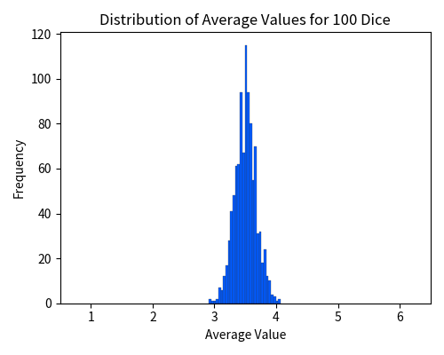
It is evident that the values are significantly concentrated around \(3.5\).

Finally, here is the case of rolling 10,000 dice. The values are so tightly concentrated around \(3.5\) that the spread is barely visible.

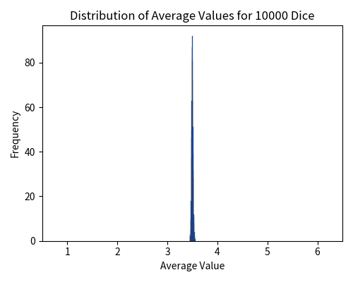
Thus, as the sample size (i.e., the number of dice) increases, the sample mean concentrates around the expected value (i.e., \(3.5\)). If the number of dice were increased infinitely, the spread would become negligible, and the sample mean would almost surely match the expected value.

In the discussion above, we have experimentally verified this concentration phenomenon, which can also be theoretically guaranteed using statistical theory, as we will see below.

Markov’s Inequality

The term concentration inequality refers to inequalities that express the concentration phenomenon. Below, we present two representative concentration inequalities — Chebyshev’s inequality and Hoeffding’s inequality. However, before doing so, we introduce Markov’s Inequality, which, although not a concentration inequality by itself, forms the basis for many of them. If you are not comfortable with mathematics, it is sufficient to understand the meaning and application of the inequality.

Markov’s Inequality expresses that the probability of obtaining a value extremely larger than the expectation is low. For example, if we set \(a = 10 \mathbb{E}[X]\), then

\begin{align}\Pr(X \ge 10 \mathbb{E}[X]) \le \frac{\mathbb{E}[X]}{10 \mathbb{E}[X]} = \frac{1}{10}.\end{align}

This indicates that the probability of \(X\) taking on a value more than 10 times its expectation is at most \(\frac{1}{10}\). This is easy to verify. If the probability of obtaining a value 10 times greater than the expectation were more than \(\frac{1}{10}\), then when computing the expectation as a weighted sum, the terms corresponding to these extreme values would alone exceed the expected value, which leads to a contradiction. Markov’s Inequality is the general statement of this observation.

Below is an appendix proof. Feel free to skip it if you prefer.

Chebyshev’s Inequality

We are ready to introduce the first concentration inequality, Chebyshev’s Inequality.

Chebyshev’s Inequality expresses that the probability of a value deviating extremely far from the expectation is low.

For example, if we set \(k = 10 \sigma\), then

\begin{align}\Pr(|X-\mu| \ge 10 \sigma) \le \frac{\sigma^2}{100 \sigma^2} = \frac{1}{100}.\end{align}

This indicates that the probability of a value being more than 10 times the standard deviation \(\sigma\) away from the expectation is at most \(\frac{1}{100}\).

Those who are somewhat familiar with statistics may have heard of the terms “2-sigma range” and “3-sigma range.” The 2-sigma range refers to the interval \([\mu – 2\sigma, \mu + 2\sigma]\), meaning values that deviate from the mean by up to twice the standard deviation \(\sigma\), while the 3-sigma range is the interval \([\mu – 3\sigma, \mu + 3\sigma]\). According to Chebyshev’s Inequality,

\begin{align} \Pr(X \in [\mu – 2\sigma, \mu + 2\sigma]) &= \Pr(|X – \mu| \le 2 \sigma) \\ &\ge 1 – \Pr(|X – \mu| \ge 2 \sigma) \\ &\stackrel{\text{(a)}}{\ge} 1 – \frac{\sigma^2}{4 \sigma^2} \\ &= 1 – \frac{1}{4} \\ &= \frac{3}{4}. \end{align}

Similarly,

\begin{align} \Pr(X \in [\mu – 3\sigma, \mu + 3\sigma]) \ge 1 – \frac{1}{9} = \frac{8}{9}, \end{align}

whrere we used Chebyshev’s Inequality in (a). We conclude that the random variable lies within the 2-sigma range with a probability of at least \(\frac{3}{4} = 75\%\), and within the 3-sigma range with a probability of at least \(\frac{8}{9} \approx 88.88\%\). The 2-sigma and 3-sigma ranges are commonly used for the normal distribution, where approximately 95.45% of the values fall within the 2-sigma range and about 99.73% fall within the 3-sigma range. Although Chebyshev’s Inequality provides a looser guarantee, its strength lies in its universal applicability — it holds for any distribution, whether normal, uniform, binomial, or even a distribution that does not fit into a specific classification. For instance, the loss distribution of a machine learning model is typically neither normal nor uniform, but often a complex distribution with no particular name. Even in such cases, Chebyshev’s Inequality can be applied to deduce that the values fall within a certain range with a specified probability. We will discuss such arguments further in the latter part of this article, so please stay tuned.

Chebyshev’s Inequality can be proven by applying Markov’s Inequality to the random variable \(Y = (X-\mu)^2\). Here, \(Y\) is a non-negative random variable whose expectation is \(\mathbb{E}[Y] = \mathbb{E}[(X-\mu)^2] = \sigma^2\). This allows us to bound the probability that \(Y\) exceeds \(\sigma^2\) using Markov’s Inequality.

Below is an appendix proof. Feel free to skip it if you prefer.

Verification of Chebyshev’s Inequality

Let’s verify Chebyshev’s Inequality in practice.

Here, we use the dice-rolling experiments discussed earlier as an example to see how Chebyshev’s Inequality can be applied. First, we compute the variance of a single die roll, then derive the variance of the sample mean, and finally apply Chebyshev’s Inequality.

Variance of a Die Roll

Since the outcome of a die, \(X\), follows a uniform distribution from 1 to 6, its expectation is\\(mathbb{E}[X] = 3.5\).

The variance can be calculated as follows:

\begin{align} \mathrm{Var}(X) &= \mathbb{E}[(X – \mathbb{E}[X])^2] \\ &= \sum_{i=1}^{6} (i – 3.5)^2 \cdot \frac{1}{6} \\ &= \frac{(1 – 3.5)^2 + (2 – 3.5)^2 + (3 – 3.5)^2 + (4 – 3.5)^2 + (5 – 3.5)^2 + (6 – 3.5)^2}{6} \\ &= \frac{6.25 + 2.25 + 0.25 + 0.25 + 2.25 + 6.25}{6} \\ &= \frac{17.5}{6} \\ &= \frac{35}{12} \approx 2.92. \end{align}

Variance of the Sample Mean

When rolling \(n = 10\) dice and taking the average of their outcomes, the variance of the sample mean

\begin{align} \bar{X} = \frac{1}{n} \sum_{i=1}^{n} X_i \end{align}

is given by

\begin{align} \mathrm{Var}(\bar{X}) &= \mathrm{Var}\left( \frac{1}{n} \sum_{i=1}^{n} X_i\right) \\ &\stackrel{(a)}{=} \frac{1}{n^2} \mathrm{Var}\left( \sum_{i=1}^{n} X_i\right) \\ &\stackrel{(b)}{=} \frac{1}{n^2} \left(\mathrm{Var}( X_1 ) + \ldots + \mathrm{Var}( X_n )\right) \\ &\stackrel{(c)}{=} \frac{1}{n} \cdot \mathrm{Var}\left( X_1 \right) \\ &= \frac{35}{12 \times 10} \\ &= \frac{35}{120} \\ &= \frac{7}{24} \approx 0.292. \end{align}

Here, (a) follows from the property \(\mathrm{Var}(aX) = a^2\,\mathrm{Var}(X)\), (b) is due to the independence of \(X_1, \ldots, X_n\), and (c) follows because \(X_1, \ldots, X_n\) are identically distributed. In other words, the variance of the sample mean \(\bar{X}\) for \(n = 10\) dice is one-tenth of the variance of a single die roll.

Application of Chebyshev’s Inequality

According to Chebyshev’s Inequality, the probability that the sample mean \(\bar{X}\) deviates from its expectation \(\mathbb{E}[\bar{X}] = 3.5\) by at least \(k\) is bounded by

\begin{align} \Pr(|\bar{X} – 3.5| \ge k) \le \frac{\mathrm{Var}(\bar{X})}{k^2}. \end{align}

Case: \(k = 1\)

\begin{align} \Pr(|\bar{X} – 3.5| \ge 1) &\le \mathrm{Var}(\bar{X}) = \frac{7}{24} \approx 0.292. \end{align}

This result indicates that the probability that the sample mean \(\bar{X}\) deviates from the expected value by at least 1 is at most 0.292.

In practice, the sample mean \(\bar{X}\) rarely deviates from the expected value by 1 or more.

In earlier experiments, the proportion of cases where the sample mean deviated by 1 or more — that is, falling outside the red dotted line — was only 0.055. Indeed, the bound of at most 0.292 seems to hold.

Case: \(k = 1.5\)

\begin{align} \Pr(|\bar{X} – 3.5| \ge 1.5) &\le \frac{7}{24 \times (1.5)^2} \\ &= \frac{7}{24 \times 2.25} \\ &= \frac{7}{54} \\ &\approx 0.1296. \end{align}

This shows that the probability that the sample mean \(\bar{X}\) deviates from the expected value by at least 1.5 is at most 0.1296.

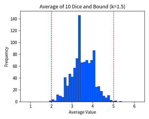
In practice, the proportion of cases where the sample mean deviates by at least 1.5 — that is, falling outside the red dotted line — is only 0.004. Indeed, the bound of at most 0.1296 seems to hold.

Case: \(n = 100\)

When rolling \(n = 100\) dice, the variance of the sample mean is one-hundredth of the variance of a single die, i.e., \(\frac{7}{240}\). Therefore, the probability that the sample mean \(\bar{X}\) deviates from its expected value by at least 1 is at most 0.0292, and the probability that it deviates by at least 1.5 is at most 0.01296. In other words, such deviations rarely occur, and it is almost certain that the sample mean \(\bar{X}\) will deviate from the expected value by less than 1. In fact, in previous experiments, not a single instance of a deviation of 1 or more was observed over 1000 trials — that is, the proportion was less than 0.001.

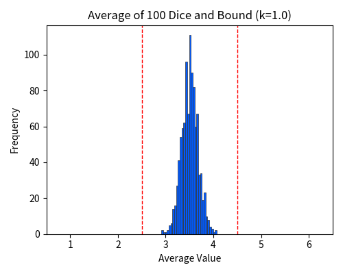
For \(n = 10\), the probability of a deviation of at least \(k = 1\) was bounded by \(\frac{7}{24} \approx 0.292\). For \(n = 100\), we have

\begin{align} \Pr\left(|\bar{X} – 3.5| \ge \frac{1}{\sqrt{10}}\right) &\le \frac{7}{240 \times \left(\frac{1}{\sqrt{10}}\right)^2} \\ &= \frac{7}{24}. \end{align}

That is, with \(k = \frac{1}{\sqrt{10}} \approx 0.316\), the same probability bound is guaranteed, and we have a narrower interval.

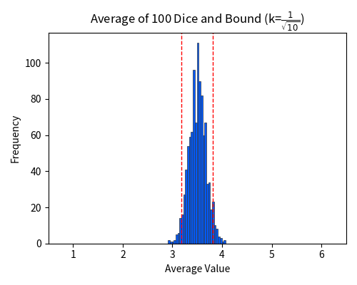
Thus, as the sample size increases, if the deviation range is fixed, the probability of falling outside that range decreases in inverse proportion to the sample size, ensuring that the sample mean almost certainly lies within the fixed range. Conversely, if we fix the probability, the interval within which the sample mean falls shrinks in inverse proportion to the square root of the sample size. This provides a theoretical proof of the concentration phenomenon.

Hoeffding’s Inequality

Although Chebyshev’s inequality is useful in a wide range of situations, it has the drawback of providing a rather loose bound for tail probabilities. For example, when rolling 100 dice, the histogram shows that a deviation of 1.5 or more from the expected value hardly ever occurs.

However, Chebyshev’s inequality somewhat pessimistically suggests that such deviations might occur with roughly a 1% probability. Tail probabilities often decay exponentially as one moves further away from the expected value, but Chebyshev’s inequality only controls them at a polynomial rate (\(\frac{1}{k^2}\)). This bound is too loose to yield useful theoretical guarantees in many cases.

To more tightly control these tail probabilities, we now introduce Hoeffding’s inequality.

When all the random variables \(X_i\) take values in the interval \([0, 1]\), Hoeffding’s inequality simplifies to

\begin{align} \Pr(|\bar{X} – \mathbb{E}[\bar{X}]| \ge t) \le 2\exp(-2nt^2). \end{align}

The key point of Hoeffding’s inequality is that the probability of a deviation from the expected value decays exponentially with both the sample size \(n\) and the deviation \(t\). Therefore, when both the sample size and the deviation are large, Hoeffding’s inequality provides a much stronger guarantee than Chebyshev’s inequality.

In the previous dice example, when \(n = 100\) and \(t = 1.5\), we have

\begin{align} \Pr(|\bar{X} – 3.5| \ge 1.5) &\le 2 \exp\left(-\frac{2n^2 t^2}{\sum_{i=1}^{n}(6 – 1)^2}\right) \\ &= 2\exp\left(-\frac{2n t^2}{25}\right) \\ &= 2\exp(-18) \\ &\approx 0.0000000304. \end{align}

This result is in excellent agreement with the observed outcomes (essentially zero). Compared to Chebyshev’s inequality — which could only bound this probability to about 1% or less — the power of Hoeffding’s inequality is clearly demonstrated.

Below, we present the proof. Those who are curious may read on; otherwise, feel free to skip it.

Model Evaluation

We are ready to discuss machine learning theory. While we will discuss model training later, let us first consider model evaluation. The loss function \(\ell(x; \theta)\) represents the loss associated with the parameter \(\theta\) for a given data point \(x\). The data \(x\) can be either supervised data — where inputs and corresponding labels are paired — or unsupervised data consisting of inputs only. In model evaluation, the loss function \(\ell\) and the parameter \(\theta\) are predetermined and remain fixed throughout the evaluation process.

We sample evaluation data \(X_1, X_2, \dots, X_n\) from a data distribution \(D\) and compute the empirical risk as follows:

\begin{align} \hat{R}_n = \frac{1}{n} \sum_{i=1}^{n} \ell\bigl(X_i; \theta\bigr). \end{align}

On the other hand, the true risk (population mean) is defined by considering not only the sampled data but all possible data:

\begin{align} R = \mathbb{E}_{X\sim D}\Bigl[\ell\bigl(X; \theta\bigr)\Bigr]. \end{align}

This population risk is an unknown constant that reflects the true quality of the model. The purpose of evaluation is to uncover this value and thereby reveal the model’s true performance.

Let us define the random variables representing the loss for each evaluation data point \(X_i\) as

\begin{align} Z_1 &= \ell\bigl(X_1; \theta\bigr), \\ Z_2 &= \ell\bigl(X_2; \theta\bigr), \\ \vdots \quad & \\ Z_n &= \ell\bigl(X_n; \theta\bigr). \end{align}

Then, the empirical risk is expressed as

\begin{align} \hat{R}_n = \frac{1}{n} \sum_{i=1}^{n} Z_i \end{align}

and the true risk is given by

\begin{align} R = \mathbb{E}[Z]. \end{align}

In the dice experiment analogy, each \(Z_i\) corresponds to the outcome of the \(i\)-th die, and the true risk \(R\) corresponds to the expected value \(\mu = 3.5\).

Similar to the dice experiment, let us now conduct an experiment in which we sample 100 evaluation data points and compute the empirical risk \(\hat{R}_n\).

We repeat this experiment 1000 times and plot the 1000 average values \(\hat{R}_n\), as shown in the figure below.

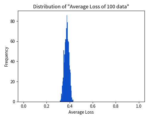
Unlike the dice experiment, where the expectation is explicitly given as \(\mu = 3.5\), the true risk \(R\) is not known beforehand. However, the figure suggests that \(R\) is approximately around \(0.37\).

Chebyshev’s inequality and Hoeffding’s inequality can be applied here just as in the dice experiment. For instance, using Chebyshev’s inequality we have

\begin{align} \Pr\Bigl(|R – \hat{R}_n| \ge k\Bigr) \le \frac{\mathrm{Var}(\hat{R}_n)}{k^2} = \frac{\mathrm{Var}(Z)}{nk^2}. \end{align}

By sufficiently increasing the number of evaluation data points \(n\), we can guarantee that, with very high probability (for example, 99.99%), the empirical risk \(\hat{R}_n\) will lie within \(k\) of the true risk \(R\). In other words, from only a finite set of evaluation data \(X_1, X_2, \dots, X_n\) that we have collected, we can infer the true risk \(R\) that applies to all data, including unseen samples.

The Same Argument Does Not Hold In Training

Next, let’s consider model training.

Assume that the loss function \(\ell\) is predetermined. In the training process, we first sample training data \(X_1, X_2, \dots, X_N\) from the data distribution. We then define the training loss as

\begin{align} \hat{R}_n(\theta) = \frac{1}{n} \sum_{i=1}^{n} \ell\bigl(X_i; \theta\bigr), \end{align}

and determine the parameter that minimizes the training loss as

\begin{align} \theta^\ast = \textrm{argmin}_{\theta} ~\hat{R}_n(\theta). \end{align}

Now, if the training loss \(\hat{R}_n(\theta^\ast)\) is low, can we conclude that the population risk

\begin{align} R(\theta^\ast) = \mathbb{E}\Bigl[\ell\bigl(X; \theta^\ast\bigr)\Bigr] \end{align}

is also low? Unfortunately, the arguments we have made so far do not allow us to say so. What is different here? The fundamental difference is that the parameter \(\theta^\ast\) is chosen after observing the data. Since \(\theta^\ast\) depends on the sample, it is itself a random variable. To emphasize its randomness, we denote it by the uppercase \(\Theta^\ast\).

In the evaluation case of the previous section, the parameter \(\theta\) was a fixed constant, so that each loss value

\begin{align} Z_1 &= \ell\bigl(X_1;\theta\bigr), \\ Z_2 &= \ell\bigl(X_2;\theta\bigr), \\ \vdots & \\ Z_n &= \ell\bigl(X_n;\theta\bigr). \end{align}

was independent. However, in the current case, even if we define \(Z_i\) as

\begin{align} Z_1 &= \ell\bigl(X_1;\Theta^\ast\bigr), \\ Z_2 &= \ell\bigl(X_2;\Theta^\ast\bigr), \\ \vdots & \\ Z_n &= \ell\bigl(X_n;\Theta^\ast\bigr). \end{align}

these loss values share the same random variable \(\Theta^\ast\) and are no longer independent. All of our previous arguments relied on independence, so if independence no longer holds, the same arguments do not apply.

Another way to view this is that the hypothesis is chosen after observing the sample. For example, if you were to predict the outcome of a die roll before tossing the die, then — without any supernatural ability — the probability of being correct is \(1/6\). This is a matter of probability. However, if you observe the die roll and then exclaim, “I knew it would be 3!” the “probability” of being correct becomes \(1\). In this way, if you choose your hypothesis after gathering the data, probabilistic guarantees based on classical probability theory no longer hold.

Thus, in model training — where the evaluation target is determined after observing the sampled data — more refined assumptions and arguments are necessary, making it far more challenging to obtain theoretical guarantees than in the case of evaluation.

Union Bound

A powerful tool that can be used even when independence does not hold is the Union Bound (also known as Boole’s inequality).

For example, suppose that the probabilities of some rare events \(E_1, E_2, E_3\) are bounded as follows:

\begin{align} \Pr(E_1) &\le \epsilon_1, \\ \Pr(E_2) &\le \epsilon_2, \\ \Pr(E_3) &\le \epsilon_3. \end{align}

Then, the probability that at least one of these events occurs is bounded by

\begin{align} \Pr\Bigl(E_1 \cup E_2 \cup E_3\Bigr) \le \epsilon_1 + \epsilon_2 + \epsilon_3. \end{align}

This result may seem obvious to many. Nevertheless, for the sake of completeness, we include a proof below; feel free to skip it if you are not interested.

When the Number of Candidates is Finite

Consider the case where there are only three candidate parameters \(\theta_1, \theta_2, \theta_3\). We consider the following training process:

1. Sample training data \(X_1, X_2, \dots, X_n\) from the data distribution.
2. Define the training loss as

\begin{align} \hat{R}_n(\theta) = \frac{1}{n}\sum_{i=1}^{n} \ell\bigl(X_i;\theta\bigr). \end{align}

3. For each candidate parameter \(\theta_1, \theta_2, \theta_3\), compute the training loss \(\hat{R}_n(\theta)\) and select the one with the lowest value:

\begin{align} \Theta^\ast = \textrm{argmin}_{\theta\in\{\theta_1,\theta_2,\theta_3\}} \hat{R}_n(\theta). \end{align}

Although in training we typically minimize the training loss \(\hat{R}_n(\theta)\) using methods such as stochastic gradient descent, the approach of computing the loss for all candidates and choosing the best one — as in this example — is also a valid form of “optimization.” Moreover, the essential aspect of the training process — selecting the parameter after seeing the data — remains intact.

It is important to note that \(\Theta^\ast\) is a random variable, as it depends on the sample, whereas the candidate parameters \(\theta_1, \theta_2, \theta_3\) are predetermined constants that exist independently of the sample. In other words, the decision to choose from the candidates \(\theta_1, \theta_2, \theta_3\) is made before observing any data.

We now apply Chebyshev’s inequality to each candidate. As before, define

\begin{align} Z_\theta = \ell\bigl(X;\theta\bigr), \end{align}

and let the population risk be

\begin{align} R(\theta) = \mathbb{E}\Bigl[Z_\theta\Bigr]. \end{align}

Then, by Chebyshev’s inequality, we have

\begin{align} \Pr\Bigl(|\hat{R}_n(\theta_1)-R(\theta_1)| \ge k\Bigr) &\le \frac{\mathrm{Var}(Z_{\theta_1})}{nk^2}, \\ \Pr\Bigl(|\hat{R}_n(\theta_2)-R(\theta_2)| \ge k\Bigr) &\le \frac{\mathrm{Var}(Z_{\theta_2})}{nk^2}, \\ \Pr\Bigl(|\hat{R}_n(\theta_3)-R(\theta_3)| \ge k\Bigr) &\le \frac{\mathrm{Var}(Z_{\theta_3})}{nk^2}. \end{align}

Applying the union bound yields

\begin{align} &\Pr\Bigl(|\hat{R}_n(\theta_1)-R(\theta_1)| \ge k \text{ or } |\hat{R}_n(\theta_2)-R(\theta_2)| \ge k \text{ or } |\hat{R}_n(\theta_3)-R(\theta_3)| \ge k\Bigr) \\ &\le \frac{\mathrm{Var}(Z_{\theta_1}) + \mathrm{Var}(Z_{\theta_2}) + \mathrm{Var}(Z_{\theta_3})}{nk^2}. \end{align}

That is, the probability that at least one of the candidate parameters has its empirical risk deviating from its true risk by at least \(k\) is small. Taking the complement, we have

\begin{align} &\Pr\Bigl(|\hat{R}_n(\theta_1)-R(\theta_1)| < k \text{ and } |\hat{R}_n(\theta_2)-R(\theta_2)| < k \text{ and } |\hat{R}_n(\theta_3)-R(\theta_3)| < k\Bigr) \\ &\ge 1 – \frac{\mathrm{Var}(Z_{\theta_1}) + \mathrm{Var}(Z_{\theta_2}) + \mathrm{Var}(Z_{\theta_3})}{nk^2}. \end{align}

This means that, in most cases, none of the candidates deviates significantly. By increasing the sample size \(n\), we can almost surely ensure that the training losses for all candidates \(\theta_1, \theta_2, \theta_3\) are close to their respective true risks. Since \(\Theta^\ast\) is chosen from among these candidates, it follows that

\begin{align} \Pr\Bigl(|\hat{R}_n(\Theta^\ast)-R(\Theta^\ast)| < k\Bigr) \ge 1 – \frac{\mathrm{Var}(Z_{\theta_1}) + \mathrm{Var}(Z_{\theta_2}) + \mathrm{Var}(Z_{\theta_3})}{nk^2}. \end{align}

Here, \(\hat{R}_n(\Theta^\ast)\) is the loss computed on the training data after training. This guarantees that, with high probability, \(\hat{R}_n(\Theta^\ast)\) is close to the true risk \(R(\Theta^\ast)\) — which considers all possible data beyond the training data points.

Since we already know from our training procedure that \(\hat{R}_n(\Theta^\ast)\) is small (because we chose \(\Theta^\ast\) as the candidate with the lowest training loss), it follows that the corresponding true risk \(R(\Theta^\ast)\) is also small, leading to good test performance.

A similar argument holds as long as the number of candidate parameters \(\theta_1, \theta_2, \dots, \theta_m\) is finite. When the number of candidates increases, tail bounds from Hoeffding’s inequality become useful. For example, as seen in the dice experiment, if we have \(n = 100\) and \(k = 1.5\), Hoeffding’s inequality gives

\begin{align} \Pr(|\bar{X} – 3.5| \ge 1.5) &\le 2\exp(-18) \\ &\approx 0.0000000304, \end{align}

so that even if there are, say, 1,000,000 candidate parameters, the union bound gives
\(0.0000000304 \times 1000000 = 0.0304\); that is, the probability of a large deviation remains around 3%. Conversely, the required sample size or allowable deviation only needs to grow logarithmically with the number of candidates. This ensures that, even with a very large number of candidates, we obtain sufficiently strong guarantees.

When the Number of Candidates is Infinite

Although Hoeffding’s inequality allows us to handle a large number of candidates, it becomes unmanageable when the number of candidates is infinite. In practice, however, parameters take continuous values (for example, in \(\mathbb{R}^d\) or \([0,1]^d\)), so there are infinitely many candidates. To deal with the infinite case, we need an additional idea: the covering number.

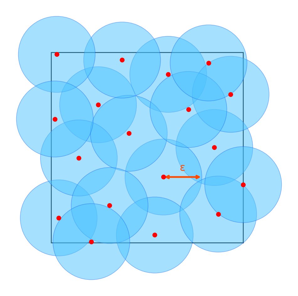
Think of an \(\epsilon\)-cover as a set of representative points. Since there are only finitely many representative points, we can apply the union bound — as in the previous section — to obtain theoretical guarantees for these points. Moreover, any point that is not one of the representatives is within \(\epsilon\) of some representative, and since we have guarantees for the representative, this ensures that the theoretical guarantee extends to all points in the set.

Let’s derive a bound under several assumptions.

First, we define the loss function \(\ell\) and randomly initialize the parameter \(\theta\). We sample training data \(X_1, X_2, \dots, X_n\) and use gradient descent (or any other optimization method) to minimize the training loss

\begin{align} \hat{R}_n(\theta) = \frac{1}{n}\sum_{i=1}^{n} \ell\bigl(X_i;\theta\bigr)\end{align}

to obtain the parameter \(\Theta^\ast\).

We now make the following assumptions:

1. Bounded Parameter Set:
   The final parameter \(\Theta^\ast\) obtained via training is assumed to lie in the set

\begin{align} \mathcal{H} = \Bigl\{\theta \in \mathbb{R}^d : \|\theta\| \le R\Bigr\}. \end{align}

This can be guaranteed through techniques such as regularization or normalization.

2. Bounded Loss:
   We assume that the loss \(\ell\) takes values in the interval \([0,1]\). This can be ensured by normalizing the scale of the loss.
3. Lipschitz Continuity:
   The loss \(\ell\) is assumed to be \(L\)-Lipschitz continuous with respect to the parameter \(\theta\). That is,

\begin{align} \|\theta_1 – \theta_2\| \le \epsilon \quad \Rightarrow \quad \bigl|\ell\bigl(X;\theta_1\bigr)-\ell\bigl(X;\theta_2\bigr)\bigr| \le L \epsilon. \end{align}

In other words, small changes in the parameter lead to only small changes in the loss.

The candidate parameter set \(\mathcal{H} = \{\theta \in \mathbb{R}^d : |\theta| \le R\}\) is contained within a \(d\)-dimensional hypercube

\begin{align} \mathcal{H}’ = \Bigl\{ \theta \in \mathbb{R}^d : |\theta_i| \le R,\; i=1,\dots,d \Bigr\}. \end{align}

Partition the hypercube \(\mathcal{H}’\) into a grid of small cubes with side length \(\frac{2\epsilon}{\sqrt{d}}\). Let \(\mathcal{C}\) be the set of centers of these small cubes. Then, \(\mathcal{C}\) forms an \(\epsilon\)-cover of \(\mathcal{H}’\) because the ball centered at each representative (with radius \(\epsilon\)) completely covers its corresponding small cube, and together they cover all of small cubes and \(\mathcal{H}’\).

The number of small cubes along each edge is

\begin{align} \left\lceil \frac{\sqrt{d}\,R}{\epsilon} \right\rceil, \end{align}

so the covering number of \(\mathcal{H}’\) (and hence \(\mathcal{H}\)) is bounded by

\begin{align} N(\mathcal{H};\epsilon) \le \left\lceil \frac{\sqrt{d}R}{\epsilon} \right\rceil^d. \end{align}

In particular, if we choose \(\epsilon = \frac{1}{4nL}\), then

\begin{align} N\left(\mathcal{H};\frac{1}{4nL}\right) \le \left\lceil 4\sqrt{d}RnL \right\rceil^d. \end{align}

Next, let \(\hat{\Theta}^\ast\) be defined as the closest point in \(\mathcal{C}\) to \(\Theta^\ast\):

\begin{align} \hat{\Theta}^\ast = \textrm{argmin}_{\theta \in \mathcal{C}} \|\Theta^\ast – \theta\|. \end{align}

By the covering property, we have

\begin{align} \|\Theta^\ast – \hat{\Theta}^\ast\| \le \epsilon. \end{align}

For each representative point \(\theta \in \mathcal{C}\), we can apply Hoeffding’s inequality in the same manner as before to obtain

\begin{align} \Pr\Bigl(|\hat{R}_n(\theta) – R(\theta)| \ge t\Bigr) &\le 2\exp\Bigl(-\frac{2n^2 t^2}{\sum_{i = 1}^n (1 – 0)^2}\Bigr) \\
&= 2\exp\Bigl(-2n t^2\Bigr). \end{align}

Using the union bound, we then have

\begin{align} \Pr\Bigl(\exists\, \theta \in \mathcal{C}:\; |\hat{R}_n(\theta)-R(\theta)| \ge t\Bigr) \le 2\,N(\mathcal{H};\epsilon)\,\exp\Bigl(-2n t^2\Bigr). \end{align}

We set

\begin{align} \epsilon &= \frac{1}{4nL}, \\[1mm] t &= \sqrt{\frac{d \log \Bigl(200 \left\lceil 4\sqrt{d}RnL \right\rceil\Bigr)}{2n}}. \end{align}

Substituting these values into the union bound gives

\begin{align}
\Pr\left(\exists\, \theta \in \mathcal{C}:\; |\hat{R}_n(\theta)-R(\theta)| \ge \sqrt{\frac{d \log \Bigl(200 \left\lceil 4\sqrt{d}RnL \right\rceil\Bigr)}{2n}}\right) \le 0.01,
\end{align}

which implies that

\begin{align} \Pr\left(\forall\, \theta \in \mathcal{C}:\; |\hat{R}_n(\theta)-R(\theta)| < \sqrt{\frac{d \log \Bigl(200 \left\lceil 4\sqrt{d}RnL \right\rceil\Bigr)}{2n}}\right) \ge 0.99. \end{align}

Thus, with at least 99% probability, the empirical risk and the true risk differ by less than \(t\) for every representative point in \(\mathcal{C}\). In particular, since \(\hat{\Theta}^\ast \in \mathcal{C}\), this guarantee holds for \(\hat{\Theta}^\ast\) as well. For the remainder of the discussion, assume that this event (i.e. the 99%-guaranteed event) holds.

Since the loss function \(\ell\) is \(L\)-Lipschitz continuous and we have \(|\Theta^\ast – \hat{\Theta}^\ast| \le \epsilon\), we obtain

\begin{align} |\hat{R}_n(\Theta^\ast)-\hat{R}_n(\hat{\Theta}^\ast)| &= \left|\frac{1}{n} \sum_i \ell(X_i; \Theta^\ast)-\frac{1}{n} \sum_i \ell(X_i; \hat{\Theta}^\ast)\right| \\ &\le \frac{1}{n} \sum_i \left|\ell(X_i; \Theta^\ast)-\ell(X_i; \hat{\Theta}^\ast)\right| \\ &\le \frac{1}{n} \sum_i \epsilon L \\ &= \epsilon L. \end{align}

Similarly,

\begin{align} |R(\Theta^\ast)-R(\hat{\Theta}^\ast)| &= \left|\mathbb{E}[\ell(X; \Theta^\ast)]-\mathbb{E}[\ell(X; \hat{\Theta}^\ast)]\right| \\ &\le \mathbb{E}\left[\left|\ell(X; \Theta^\ast)-\ell(X; \hat{\Theta}^\ast)\right|\right] \\ &\le \mathbb{E}[\epsilon L] \\ &= \epsilon L. \end{align}

By the triangle inequality,

\begin{align}
&|\hat{R}_n(\Theta^\ast)-R(\Theta^\ast)| \\ &\le |\hat{R}_n(\Theta^\ast)-\hat{R}_n(\hat{\Theta}^\ast)| + |\hat{R}_n(\hat{\Theta}^\ast)-R(\hat{\Theta}^\ast)| + |R(\Theta^\ast)-R(\hat{\Theta}^\ast)| \\
&\le \epsilon L + t + \epsilon L \\
&= 2\epsilon L + t \\
&= \frac{1}{2n} + \sqrt{\frac{d \log \Bigl(200 \left\lceil 4\sqrt{d}RnL \right\rceil\Bigr)}{2n}} \\
&\le 2 \sqrt{\frac{d \log \Bigl(200 \left\lceil 4\sqrt{d}RnL \right\rceil\Bigr)}{2n}},
\end{align}

where the last inequality holds asymptotically or when the numerator is at least 1.

Thus, with high probability, the training loss computed on the training data, \(\hat{R}_n(\Theta^\ast)\), is guaranteed to be close to the population risk \(R(\Theta^\ast)\), which considers all data, not just the training set.

From this bound, several insights can be drawn. First, to obtain a useful bound (i.e. a right-hand side less than 1), the number of training samples \(n\) must be on the order of or larger than the dimensionality \(d\) of the parameters. If the number of samples is smaller than the number of parameters, the parameter becomes underdetermined, which is intuitively clear. The bound decreases roughly in inverse proportion to the square root of \(n\). Roughly speaking, if you have 100 times as many data points as the number of parameters, then the difference between the training performance and the test performance will be on the order of \(\sqrt{\frac{1}{100}} = \frac{1}{10}\).

Towards Deep Learning Theory

What we have discussed so far constitutes the classical learning theory. In deep learning, however, the number of parameters can range from millions to billions, and overparameterization is common — the parameter dimensionality \(d\) typically exceeds the number of training samples \(n\). As we saw in the previous section, when \(d > n\) the bound becomes greater than 1, rendering it meaningless as a guarantee. This is one of the reasons why classical learning theory fails to explain why deep learning works so well. In the overparameterized regime of deep learning, providing useful guarantees on test accuracy is an active research topic. Here, we see one possible approach.

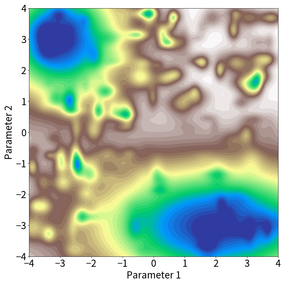
The loss landscape of a deep neural network, as shown in the figure above, consists of vast basins and sharp valleys. It is known that when training with stochastic gradient descent, the optimization almost surely escapes from the sharp valleys and converges to one of the vast basins. Well-trained models continue to perform well even if they are quantized or reduced in precision. This indicates that it is not necessary to have the exact parameter \(\theta\); rather, as long as the parameter lies within a certain range, the loss remains low — evidence that the solution resides in a wide basin. We assume that the final parameter does not remain trapped in a sharp valley but always converges to a wide basin. One can ensure this condition by restarting optimization until it converges to a basin If a model falls into a sharp valley.

Within a basin, the loss does not change significantly even if the parameters move in any direction. Therefore, selecting a single representative point in the basin is sufficient. Moreover, the number of vast basins is not very large. It has been argued that, in practice, stochastic gradient descent essentially reaches only one basin (which is why simple parameter averaging can work for model merging), or that even if there are several basins, it has been hypothesized that there is essentially a one-to-one correspondence between the basins and the way of inference, and there are few ways of inference that work well — even if there are a number of ways of inference that do not work well — there are few basins that can be reached after learning.

It is a rather coarse argument, but if we can assume that the number of basins is a constant \(K\) and that it converges to one of these \(K\) basins every time, regardless of the sample, we can use an argument analogous to the previous section to guarantee, with probability

\begin{align} 1 – 2K \exp\Bigl(-2n t^2\Bigr), \end{align}

that the error is at most

\begin{align} t + \text{(variation of the loss within the basin)}. \end{align}

If we set

\begin{align} t = \sqrt{\frac{\log(200K)}{2n}}, \end{align}

then with 99% probability the error is at most

\begin{align} \sqrt{\frac{\log(200K)}{2n}} + \text{(variation of the loss within the basin)}. \end{align}

Notably, this bound does not depend on the parameter dimension \(d\).

Whether the number of essential basins is truly a constant and under what conditions this property holds remains an open question. However, if you have followed the discussion up to this point, you can appreciate that if such properties were fully understood, then by applying the arguments above, it would be possible to provide theoretical guarantees on the test loss in deep learning as well. If you grasp these ideas, further research in this area is well within your reach. Please, give it some thought.

Author Profile

If you found this article useful or interesting, I would be delighted if you could share your thoughts on social media.

New posts are announced on @joisino_en (Twitter), so please be sure to follow!

Ryoma Sato

Currently an Assistant Professor at the National Institute of Informatics, Japan.

Research Interest: Machine Learning and Data Mining.

Ph.D (Kyoto University).

View Profile