Speculative Decoding Explained

“Generating…”
We are all familiar with the cursor blinking, slowly revealing text word by word. Whether it’s ChatGPT or a local LLM, the generation speed of autoregressive models based on Transformers is fundamentally bound by their sequential nature. It computes, emits one token, computes again, emits the next token, and repeats. This strict dependence chain introduces latency at every single step. Even on a powerful GPU, you cannot fully exploit parallel computation because the next token depends on the previous one.

So here is the punchline:
You can reduce decoding latency without changing the output distribution, without any additional training, and with an implementation that is surprisingly straightforward.

That technique is speculative decoding [Leviathan+ 2023, Chen+ 2023].

What is speculative decoding?

Speculative decoding is a technique designed to reduce the latency of autoregressive language models based on Transformers. It has three key advantages:

(1) It is an exact method that does not alter the output distribution.
(2) It requires no additional training and can be applied directly to existing models.
(3) It is easy to implement.

You accelerate a heavy model by pairing it with something lighter:

• Target model: the large model you actually want to sample from.
• Draft model: a lightweight helper model that proposes candidate tokens.

The draft model can be any type of model, such as a small Transformer, a Recurrent Neural Network, or even an n-gram model.

The pain point: why decoding is slow in the first place

In an autoregressive Transformer, each token must be generated sequentially: compute logits, sample or select a token, append it, compute again, and repeat. That sequential dependency introduces latency at every step. Even on a GPU, you cannot fully exploit parallelism when your control flow is “one token at a time.”

Speculative decoding attacks exactly this bottleneck. Instead of waiting for the target model to produce every next token, you ask a cheap draft model to propose multiple tokens quickly, then you use the target model’s parallel computation to verify them efficiently. This is the central idea.

The core loop: draft fast, verify in parallel

Fix a parameter \(\gamma\), the number of draft tokens you will propose at a time. The draft model generates \(\gamma\) tokens: \(x_1, x_2, \ldots, x_\gamma\). Then the target model verifies these tokens in parallel.

Now comes the accept/reject logic that makes everything work:

If \(x_1, \ldots, x_i\) are accepted but \(x_{i+1}\) is rejected by the target model, then \(x_1, \ldots, x_i\) and the \((i+1)\)-th token \(x’_{i+1}\) produced by the target model are confirmed.

If all \(x_1, \ldots, x_\gamma\) are accepted, then \(x_1, \ldots, x_\gamma\) and the \((\gamma+1)\)-th token \(x’_{\gamma+1}\) from the target model are confirmed.

Generation continues by conditioning on the confirmed prefix (for example, \(x_1, \ldots, x_i, x’_{i+1}\)) and repeating the same pattern.

Why this helps on GPUs

Autoregressive generation forces sequential dependence: token \(t\) must be generated before token \(t+1\). This sequential nature prevents full utilization of parallel computation capabilities, even with GPUs.

Speculative decoding breaks the bottleneck by:

• quickly generating candidates using the lightweight draft model, and
• leveraging parallel computation for efficient verification with the heavier target model.

This is not just a paper trick

Speculative decoding has been reported by Google to be in practical use in production systems, such as the AI Overviews feature displayed at the top of Google Search results [Leviathan+ 2024].

Now let us go deeper. The rest of this article presents a representative technique called speculative sampling [Leviathan+ 2023, Chen+ 2023], and then walks through several important extensions.

Speculative sampling: exact sampling from the target distribution

Let the target model’s distribution be denoted as \(p_t\), and the draft model’s distribution over continuations as \(q_d\). The goal is to sample efficiently from the distribution \(p_t\) of the target model.

Given the output \(x_1, \ldots, x_\gamma \sim q_d\) of the draft model, you might try the most naive verification strategy:

• sample \(x_1′, \ldots, x_\gamma’ \sim p_t\) as well, and
• accept \(x_i\) only if it matches, \(x_i = x_i’\); otherwise reject.

However, this fails spectacularly even when the draft model is perfect. Suppose:

\[ p_t(x) = q_d(x) = \text{Unif}(\{1, \ldots, 100\}). \]

Here, \(q_d\) exactly matches \(p_t\). And yet, if you independently sample from \(p_t\), the probability that \(x_i = x’_i\) is only 1%. That means you reject 99% of the time. With such a rejection rate, the naive approach cannot produce any meaningful speedup.

So what do you do instead? Surprisingly, you can design a verification rule that yields high acceptance when \(q_d\) is close to \(p_t\), and that becomes always accept when \(p_t = q_d\). That is exactly what speculative sampling gives you.

The speculative sampling procedure (step by step)

In speculative sampling, you first sample \(\gamma\) tokens from the draft model: \(x_{: \gamma} \sim q_d(x_{: \gamma})\). Then you input these tokens to the target model, and compute (in parallel) the conditional probabilities \(p_t(x_i \mid x_{:i-1})\) for \(i = 1, \ldots, \gamma + 1\). Note that \(p_t(x_i \mid x_{:i-1})\) can be computed in parallel since \(x_{: \gamma}\) are already at hand.

Now, for each position \(i\), you decide whether to accept the draft token \(x_i\) using the following rules:

(1) If \(q_d(x_i \mid x_{:i-1}) \le p_t(x_i \mid x_{:i-1})\), then \(x_i\) is accepted.

(2) Otherwise, sample \(r \sim \text{Unif}(0, 1)\), and accept \(x_i\) if:

\[ r < \frac{p_t(x_i \mid x_{:i-1})}{q_d(x_i \mid x_{:i-1})}. \]

For later reference in this post, call this the “SpecJudge” inequality.

(3) If the token is not accepted, it is rejected, and a new token \(x’_i\) is sampled from:

\[ \text{normalize}(\max(0,\; p_t(x_i \mid x_{:i-1}) – q_d(x_i \mid x_{:i-1}))). \]

Call this the “SpecNormalize” residual distribution.

If accepted, you move on to \(i+1\). If rejected, the process halts, and generation is resumed using the draft model, conditioned on the sequence of confirmed tokens up to that point.

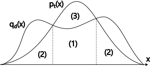
Why this is exact: the decomposition view

Intuitively, steps (1), (2), and (3) correspond to a decomposition like the figure above. But you do not have to take this on faith. You can verify precisely that the accepted token distribution equals \(p_t\).

Define the set:

\[ \mathcal{D} = \{x \mid q_d(x_i \mid x_{:i-1}) > p_t(x_i \mid x_{:i-1})\}. \]

Now consider two cases.

(i) For tokens \(x_i \in \mathcal{D}\): the token is generated by the draft model with probability \(q_d(x_i \mid x_{:i-1})\), and accepted with probability \(\frac{p_t(x_i \mid x_{:i-1})}{q_d(x_i \mid x_{:i-1})}\) due to step (2). So the acceptance probability becomes:

\[ q_d(x_i \mid x_{:i-1}) \cdot \frac{p_t(x_i \mid x_{:i-1})}{q_d(x_i \mid x_{:i-1})} = p_t(x_i \mid x_{:i-1}). \]

(ii) For tokens \(x_i \not\in \mathcal{D}\): the token is generated by the draft model with probability \(q_d(x_i \mid x_{:i-1})\), and always accepted due to step (1). Additionally, when the draft model generates a token in \(\mathcal{D}\), it is rejected with probability:

\[ C = \int_{\mathcal{D}} \left(1 – \frac{p_t(x_i \mid x_{:i-1})}{q_d(x_i \mid x_{:i-1})} \right) \text{d}x_i \]

and a new token is sampled from:

\[ \frac{p_t(x_i \mid x_{:i-1}) – q_d(x_i \mid x_{:i-1})}{C} \]

due to step (3). Therefore, the total acceptance probability is:

\[ q_d(x_i \mid x_{:i-1}) + C \cdot \frac{p_t(x_i \mid x_{:i-1}) – q_d(x_i \mid x_{:i-1})}{C} = p_t(x_i \mid x_{:i-1}). \]

In either case, the token is accepted with probability \(p_t(x_i \mid x_{:i-1})\). So the procedure is exact: you are still sampling from the target model distribution.

This resembles rejection sampling, but there is a crucial operational difference. Standard rejection sampling may reject repeatedly. Here, the token is guaranteed to be resolved in at most three steps: (1) accept directly, (2) accept via SpecJudge, or (3) reject and sample once from the SpecNormalize residual.

So does it actually speed things up?

Exactness is nice, but you care about wall-clock time. So what happens in practice?

Leviathan et al. [Leviathan+ 2023] evaluated speculative decoding using:

• Target model: T5-XXL (11B parameters)
• Draft model: T5-Small (77M parameters)

On tasks such as translation and summarization, with \(\gamma = 5\) and \(\gamma = 7\), they observed speedups of 2.3x to 3.4x. In those experiments, the per-token acceptance probability (draft token accepted by target) ranged from 53% to 75%.

Even more interestingly, you can get value from an almost trivial draft model. When using a bigram model as the draft model, an acceptance rate of about 20% was achieved, producing a 1.25x speedup at \(\gamma = 3\). Since a bigram model costs virtually nothing to run, pairing it with parallel verification can still yield meaningful acceleration. That is one of the cleanest “you might not expect this” aspects of speculative decoding.

Extensions: better drafts, online adaptation, and removing the “two-model” burden

At this point you might ask: “If the draft model can be anything, how should I choose it?” That question has driven a lot of follow-up work.

Any model can be used as the draft model, and many improvements have been proposed by carefully selecting or designing the draft model.

DistillSpec: align the draft to the target via distillation

DistillSpec [Zhou+ 2024] aligns the draft model with the target model through distillation. In conventional speculative decoding, the draft and target models are independent, and acceptance depends on how closely the draft distribution matches the target distribution.

A subtle point that can surprise you: higher token prediction accuracy of the draft model does not always lead to better results. In extreme cases, if the draft model has higher prediction accuracy than the target model, the draft may propose tokens that the target model cannot predict well. Those tokens will be rejected, and you get no speedup.

DistillSpec addresses this by distilling from the target model to the draft model so that the draft distribution approximates the target distribution. This increases acceptance probability. Reported results show a further 10% to 45% speedup over standard speculative decoding.

Online Speculative Decoding: fine-tune the draft on the fly

Online Speculative Decoding [Liu+ 2024] takes a different approach. After verifying draft outputs, the draft model is continuously fine-tuned on the fly to adapt to changes in the query distribution.

Each time a discrepancy between draft and target is observed, the target model’s output is stored in a training buffer and used as training data. This is important because it avoids significant cost for preparing training data. If your user queries are biased toward a specific domain, this online adaptation can increase acceptance rates in that domain, leading to overall speedup.

Reducing deployment overhead: folding draft and target into one model

A practical pain point of the original framework is that you must prepare and deploy two models (target and draft). Several methods integrate the draft and target roles into a single model.

Draft & Verify: truncate the target model

Draft & Verify [Zhang+ 2024] uses a truncated version of the target model (removing some layers) as the draft model.

Many modern language models employ skip connections of the form:

\[
x^{(l+1)} = x^{(l)} + f^{(l)}(x^{(l)}).
\]

Models with skip connections typically exhibit small changes in representations across layers [Liu+ 2023], so removing some layers does not significantly degrade accuracy.

There is a trade-off:

• removing more layers increases the speed of the draft model,
• but it lowers the acceptance rate.

Draft & Verify uses Bayesian optimization to search for the optimal combination of layers to remove so that end-to-end decoding speed is minimized. A key practical benefit: only a single model needs to be deployed. Experiments report up to a 1.99x speedup.

LayerSkip: predict tokens at intermediate layers without wasting compute

LayerSkip [Elhoushi+ 2024], similar to early exit models, trains the model so that token prediction is possible at any layer, and then uses the output from an intermediate layer as the draft.

During target model computation, the model starts from the layer following the draft output, so the computation done by the draft model is not wasted. Experiments have demonstrated a maximum speedup of 2.16x using this approach.

Verifying multiple candidates at once: trees, forests, and tree attention

So far, you have imagined a single draft continuation. But what if you verify multiple candidate continuations simultaneously? This increases the probability that at least one candidate will be accepted. There are methods that verify multiple draft candidates at once [Miao+ 2024; Speector+ 2023; Fu+ 2024].

Of course, verifying more candidates can increase computation time. To mitigate this cost, it has been proposed to:

• leverage parallel computation, and
• represent candidate sets using trees (or forests) and apply tree attention for efficiency.

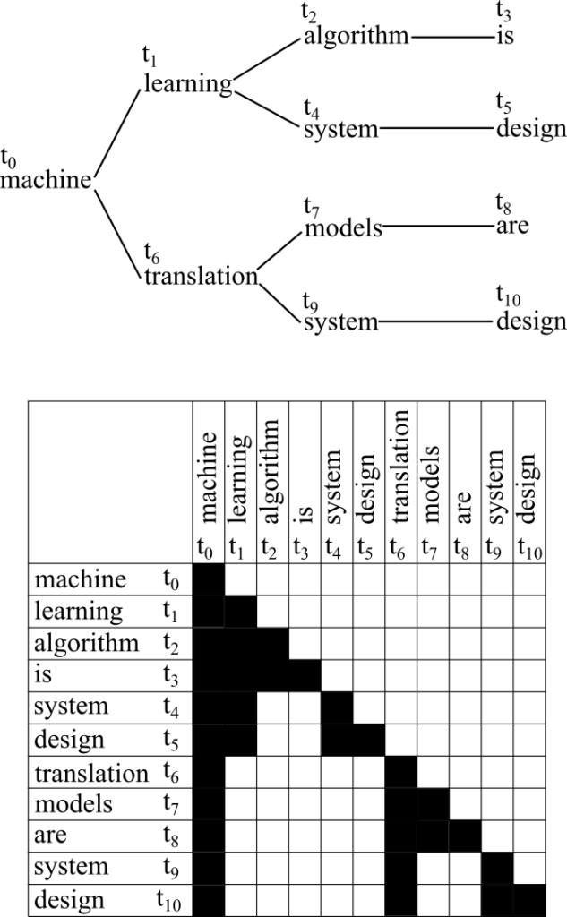
You can obtain multiple draft candidates in several ways: sample from multiple draft models, sample multiple times from a single draft model, or take top-K outputs from a draft model. Suppose you obtain the following four candidates:

(1) machine learning algorithm is
(2) machine learning system design
(3) machine translation models are
(4) machine translation system design

These can be represented as a tree consisting of 11 nodes (as in the figure). When the target model verifies these candidates, it uses an attention mask so each token attends only to ancestor nodes.

A concrete example: the token \(t_8(\text{are})\) attends only to \(t_0(\text{machine})\), \(t_6(\text{translation})\), and \(t_7(\text{models})\). Other tokens are included in the input but do not affect the result. This allows candidate (iii), “machine translation models are”, to be processed simultaneously with the others.

The accept/reject decision as a tree traversal

The accept/reject decision is repeated by traversing the tree from the root node, using the same SpecJudge inequality as above. The procedure is:

Set a pointer to the current node, starting at the root.

If the current node has multiple children (candidate next tokens), verify one candidate using the SpecJudge inequality.

If it is accepted, confirm the token and move the pointer to that node.

If it is rejected, discard that node and all descendants, renormalize the target probabilities using the SpecNormalize residual, then evaluate the next sibling.

If all children of the current node are rejected, sample one token from the remaining (renormalized) target distribution and end the process.

When there is only one candidate, the tree degenerates into a path, and this reduces to standard speculative decoding. In other words, tree attention is a generalization of standard speculative decoding. And importantly, similarly to speculative decoding, this approach does not change the distribution; this is stated as Theorem 4.2 in [Miao+ 2024].

Medusa: generate many draft candidates inside one model

Medusa [Cai+ 2024] is a method to generate multiple candidates efficiently. Instead of maintaining a separate draft model, Medusa adds additional heads to the final hidden layer of a pre-trained language model: one head predicts the token two steps ahead, another predicts three steps ahead, and so on, up to a head predicting the token \(K\) steps ahead.

These heads are trained via self-distillation so that they predict the outputs of the base model. Depending on your training budget, you can train only the heads, the entire model, or the entire model using parameter-efficient fine-tuning.

During generation:

• the head predicting the next token produces \(s_1\) candidates,
• the head for two tokens ahead produces \(s_2\) candidates,
• and so on, up to \(s_K\) candidates from the head for \(K\) tokens ahead.

These are combined to form a total of \(s_1 \cdot s_2 \cdot \ldots \cdot s_K\) candidate sequences of length \(K\), which are then used for verification by the target model using the tree attention mechanism described above.

Medusa has two advantages:
(i) only a single model needs to be maintained, and
(ii) many draft candidates can be generated in parallel.

Summary: The Era of “Lossless” Speed

Speculative decoding is not a heuristic. It is one of the rare techniques that is simultaneously: exact, training-free, and implementable with a clean decoding loop.

• Surprise 1: You can speed up LLMs significantly without changing the output quality at all (Exact method).
• Surprise 2: Even a “dumb” draft model (like a bigram) provides a speed boost because verification is parallel.
• Surprise 3: Real systems report 2.3x to 3.4x speedups with acceptance rates of 53% to 75% [Leviathan+ 2023].

The limitation of sequential generation is not an unbreakable law of physics. It is an engineering hurdle that is being cleared with elegant theoretical insights.

After seeing all of this, do you still want to accept token-by-token latency as inevitable?

Speculative decoding is not just about speed; it’s about unlocking the true potential of the hardware we already possess.

Author Profile

If you found this article useful or interesting, I would be delighted if you could share your thoughts on social media.

New posts are announced on @joisino_en (Twitter), so please be sure to follow!