One Training Example Is All You Need for Reasoning

To improve reasoning ability, it may be enough to use only one training example in the post-training of an LLM. In this post, I explain a study on reinforcement learning that uses just a single training example, “Reinforcement Learning for Reasoning in Large Language Models with One Training Example” [Wang+ NeurIPS 2025].

Intuitively, the main takeaway of this work is: if you make an LLM repeatedly think through how to solve one carefully chosen math problem, you can obtain strong reasoning ability. You do not need to prepare a wide variety of problems as in conventional training. With training on only one problem, accuracy on the MATH500 benchmark improved from 36.0% to 73.6%, and the average accuracy across six math benchmarks improved from 17.6% to 35.7%.

The training procedure is almost the same as standard reinforcement learning, but one distinctive feature is the use of a regularizer that increases the entropy of the LLM’s output distribution, that is, it encourages diverse outputs. This is expected to help the model consider alternative solutions to the same problem and recover when its thinking goes off track.

Below I describe the method and the experimental setup in detail.

We start with a pretrained LLM. This is a model right after pretraining, without instruction tuning or reinforcement learning.

We consider improving this model’s math ability via reinforcement learning. In reinforcement learning, we essentially give the LLM a problem, have it output intermediate reasoning and an answer, and then: if the answer is correct we give reward and increase the probability of producing that output; if the answer is incorrect we give a penalty and decrease the probability of producing that output.

First, we carefully select the data used in the final training. To do this, we apply conventional reinforcement learning using the full dataset (1209 math problems). During this training process, we define a problem as “good” if it has high reward variance, that is, a problem for which the LLM experiences many successes and many failures. Conversely, problems that the LLM keeps getting wrong, or keeps getting right, are not considered good. Using this criterion, we rank the problems and determine the best one, \(\pi_1\). This gives us a single carefully selected math problem to use in the final training.

Although we trained a model during this selection process, we discard it. This may look roundabout, but the goal is to study what happens when we train on a carefully selected problem, so we invest effort in selection. In practice, it would be counterproductive to train a model just to choose training data, so one might use a simpler criterion or have humans create one high-quality problem. As I discuss later, the one-example training still works even when the selection criterion is loosened to some extent.

In the paper’s experiments, the selected math problem \(\pi_1\) was the following:

The pressure P exerted by wind on a sail varies jointly as the area A of the sail and the cube of the wind’s velocity V. When the velocity is 8 miles per hour, the pressure on a sail of 2 square feet is 4 pounds. Find the wind velocity when the pressure on 4 square feet of sail is 32 pounds. Let’s think step by step and output the final answer within \boxed{}.

Computing a cube root is somewhat tricky, but this is an elementary algebra problem.

Now that we have a single carefully selected math problem, we make the LLM solve this problem over and over again.

Using \(\pi_1\) as the prompt, we generate multiple responses with different random seeds. Because LLM generation is stochastic, we get diverse outputs. Some will be correct and some will be incorrect. We reward the correct responses to increase their generation probability, and penalize the incorrect responses to decrease their generation probability. We repeat this endlessly: give the same problem \(\pi_1\), generate multiple responses, increase the probability of good ones; then again the same problem; then again the same problem. In conventional training, each round uses different data, but here every round uses the same data point \(\pi_1\). Also, as mentioned above, we use a regularizer that increases entropy and thus promotes output diversity. This encourages diverse solutions even for the same input problem, which can plausibly provide benefits such as: (i) training progresses without collapsing to only correct or only incorrect outputs, (ii) the model can learn many alternative solution paths for the same problem, and (iii) the probability of producing mistakes or tangential text increases, but the model can learn a policy that still returns to correct reasoning and ultimately reaches the correct answer to obtain reward.

Let us now look at the experimental results.

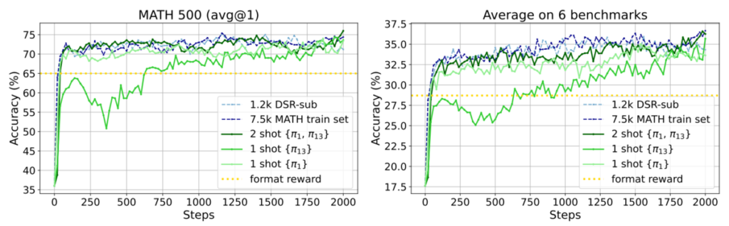
The figure above shows the main accuracy curves. The light-green line is reinforcement learning using only one problem, and it reaches accuracy comparable to the full-data reinforcement learning shown by the light-blue dotted line. The dark-green line corresponds to using not the top-ranked high-variance problem \(\pi_1\), but the 13th-ranked problem \(\pi_{13}\); this also ultimately reaches accuracy comparable to full-data training. Using two problems, \(\pi_1\) and \(\pi_{13}\), makes the intermediate trajectory closer to the full-data case.

At the beginning I said that MATH500 accuracy improved from 36.0% to 73.6%, and the average accuracy across six math benchmarks improved from 17.6% to 35.7%. The dramatic “doubling” is partly due to a trick: the baseline accuracy is measured on a model right after pretraining, with no instruction tuning at all. Such a model often has nontrivial math ability, but it frequently fails to follow instructions like “Write the final answer inside \boxed{}.” It may output the answer without boxing it, and then it is judged incorrect. In that situation, we cannot tell whether the model lacks math ability or merely fails to follow the required format.

So the authors apply a reinforcement learning procedure that teaches the model to follow the format: they reward outputs that match the format and penalize outputs that do not match the format, regardless of whether the answer is correct. The accuracy after this “format-only” reinforcement learning corresponds to the yellow dotted line in the figure above. Simply enforcing the format increases MATH500 accuracy from 36.0% to 65.0%, and the average across six math benchmarks from 17.6% to 28.7%. This shows that the pretrained model already has some math ability, and that enforcing the format reveals it. However, this does not eliminate the effect of the one-problem reinforcement learning: training on one carefully chosen math problem still provides substantial additional gains.

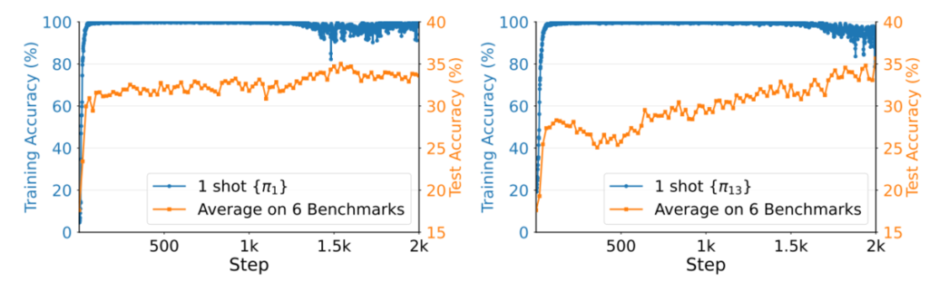
The figure above plots training accuracy and test accuracy. Training accuracy immediately becomes 100%, which is expected because there is only one training example. The puzzling parts are: even after training accuracy reaches 100%, continuing training gradually increases test accuracy, and continuing training causes training accuracy to decrease slightly and become unstable. I will explain this shortly.

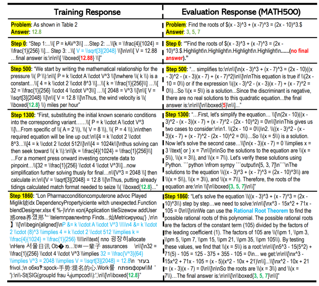
The figure above shows example outputs over time. At step 1860, where the earlier plot shows a drop in training accuracy, the output becomes chaotic, with Hangul and garbled text mixed in. As a result, even though the model has been trained on \(\pi_1\) repeatedly, it occasionally fails on this training problem. This explains why the training accuracy decreases after long training. Still, in more than 90% of trials it ultimately reaches the correct answer. Even in the step-1860 example, the model produces irrelevant text and Hangul, but it repeatedly returns to the original reasoning (highlighted in light blue) and finally arrives at the correct answer. This can be interpreted as the model acquiring a robust ability to reach the correct answer even under difficult conditions where its reasoning becomes disorganized.

Moreover, for the unseen test problem on the right, the model produces a coherent derivation and reaches the correct answer without collapsing into Hangul or garbled text.

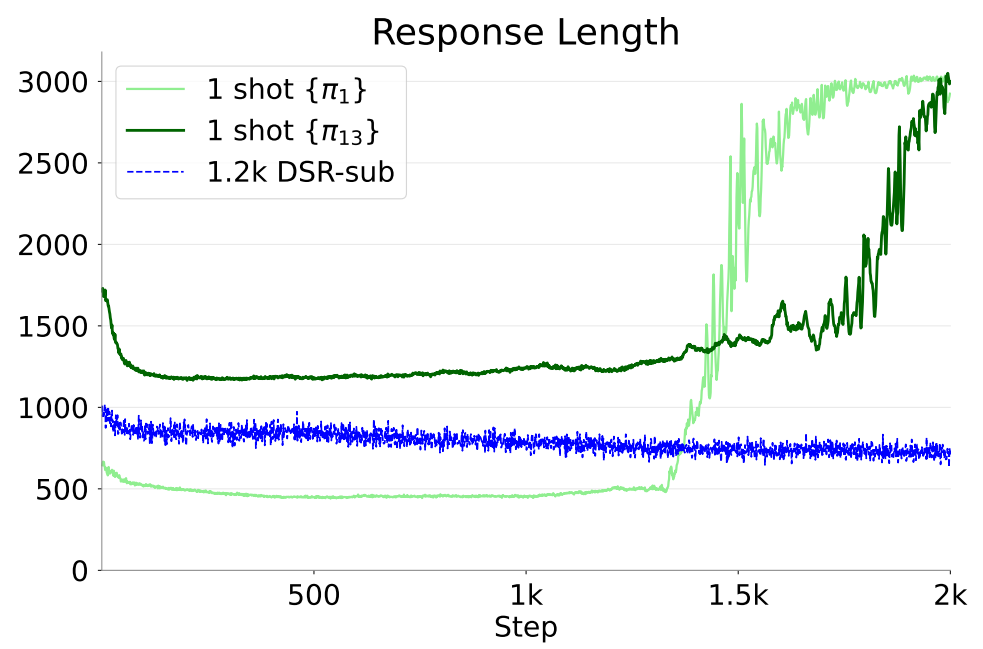
During this training process, the chain-of-thought length gradually increases, and at some point it increases sharply. This means the model starts tackling the single problem with much longer chains of thought.

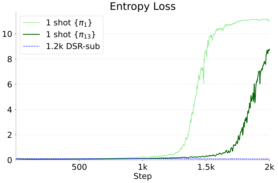
Entropy also gradually increases, then sharply increases at some point, leading to extremely diverse outputs. When there is only one training problem, the model’s accuracy on that problem quickly becomes close to 100%. From there, the only way to further reduce the overall objective is to increase the entropy term in the regularizer. Thus, the model keeps the problem solvable at near 100% while gradually increasing entropy. Then, at some point, it acquires the ability to return to the original reasoning and answer correctly even when its chain of thought collapses. At that point, it can make entropy extremely large while keeping accuracy near 100%. This explains why continued training slightly reduces training accuracy while improving test performance.

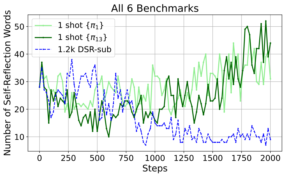
In the figure above, the green line shows how often the model outputs so-called “self-reflection words” such as “rethink,” “recheck,” and “recalculate” when trained on a single example, and this frequency increases during training. By using such words, the model can return to the original reasoning even when its thinking collapses. In other words, once the model acquires these self-reflection words, it becomes more robust to collapse and can tolerate higher entropy. Put differently, in an environment that applies pressure to increase entropy, the model acquires these self-reflection words and becomes resistant to collapse of reasoning. As a result, once it learns these self-reflection words, it becomes more reliable at reaching correct answers on general problems as well.

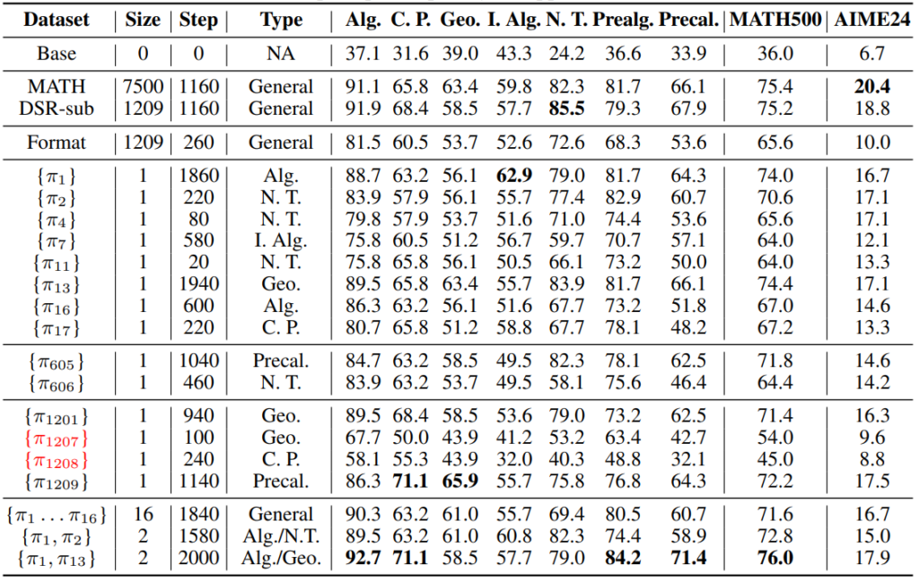
The table above shows test accuracy when different problems are used for one-example training. The performance varies somewhat, but it is clear that training on just one problem can substantially improve math ability for many choices. The exceptions, shown in red, are \(\pi_{1207}\) and \(\pi_{1208}\): one has an incorrect label, and the other is so difficult that the LLM cannot solve it at all. As long as we avoid such problems, one can obtain strong reasoning ability by training thoroughly on just a single problem, regardless of which problem it is.

Why is one training example enough? Typical pretraining uses on the order of billions of documents, so compared to that, one example is far too small. The key factor is that training to acquire knowledge and training to acquire reasoning ability are qualitatively different. To acquire knowledge, you inevitably need to show the model many data points; knowledge acquisition requires massive amounts of data, such as billions of examples. In contrast, to acquire reasoning ability, the model does not need to see an enormous number of problems; it can develop thinking ability by repeatedly working through a small number of high-quality problems. This work can be seen as presenting this difference in an extreme and easy-to-understand setting.

In practice, the ability to acquire habits like “rethink,” “recheck,” and similar self-reflection words is likely the key. Developing a habit of using such self-reflection words is a general technique that contributes to accuracy on many reasoning benchmarks. If you keep working on a single problem, you can naturally discover the usefulness of these words. Conversely, one can also interpret this as saying that, with current techniques, the kinds of abilities we can add to an LLM via post-training are limited to roughly this level, and for that level it is not necessary to prepare thousands of problems; one carefully used problem is enough.

Research on reinforcement learning to improve an LLM’s reasoning ability is very active, and I feel this paper is a good contribution because it introduces a new perspective into this line of work in a clear and accessible form. There are still many unknowns about what “reasoning ability” in an LLM really is and how to reliably induce it. I hope this post helps your understanding of LLM reasoning ability.

Author Profile

If you found this article useful or interesting, I would be delighted if you could share your thoughts on social media.

New posts are announced on @joisino_en (Twitter), so please be sure to follow!