Model Merge Explained: Build Models without Training

We can flatten the parameters of a deep neural network into a single vector. For a large model, this vector can easily have tens of billions of dimensions. At first glance it may look like a meaningless list of numbers, but it has become clear that this vector has deep meaning as a vector. For example, let \(\boldsymbol{\theta}_1\) and \(\boldsymbol{\theta}_2\) be two different parameter vectors. Then a model whose parameters are

\[
\boldsymbol{\theta}_3 = \frac{\boldsymbol{\theta}_1 + \boldsymbol{\theta}_2}{2}
\]

or

\[
\boldsymbol{\theta}_4 = 2\boldsymbol{\theta}_1 – \boldsymbol{\theta}_2
\]

still works properly. Methods that use arithmetic on model parameters are attractive in both speed and cost, because they can produce a model with desired capabilities using only simple arithmetic, without expensive training such as gradient-based optimization. In this section, we explain such methods based on model-parameter arithmetic and the theory behind them.

Model Soup

Model soup [Wortsman+ 2022] is a method that improves performance by averaging multiple sets of model parameters. Start from a pretrained model \(\boldsymbol{\theta}_0 \in \mathbb{R}^d\), and let \(\boldsymbol{\theta}_1, \boldsymbol{\theta}_2, \ldots, \boldsymbol{\theta}_n \in \mathbb{R}^d\) be the parameters obtained by training (fine-tuning) with various hyperparameter settings. For example, you may fine-tune with different choices of learning rate, weight decay, number of training iterations, data augmentation, and the strength of label smoothing, and obtain \(\boldsymbol{\theta}_1, \boldsymbol{\theta}_2, \ldots, \boldsymbol{\theta}_n\). The averaged vector

\[
\boldsymbol{\theta}_{\text{unif}} = \frac{\boldsymbol{\theta}_1 + \boldsymbol{\theta}_2 + \ldots + \boldsymbol{\theta}_n}{n}
\]

often achieves higher performance than any individual model and is more robust to distribution shift. Mixing models by averaging the parameters obtained from training under various hyperparameters is called a model soup. More generally, integrating multiple models into a single model is called a model merge.

In a typical training workflow, after training with various hyperparameters, you evaluate on validation data, keep only the best model, and discard the rest. The advantage of model soup is that it can use those models that would otherwise be discarded as ingredients to improve performance. It requires no additional training time. Another attractive point is that it does not require a validation dataset.

Model soup is similar to ensembling, but it differs greatly in inference time and deployment simplicity. If you ensemble \(n\) models, inference time becomes \(n\) times larger. With model soup, inference time is usually unchanged from a standard single model. In deployment, ensembles are cumbersome because you must manage multiple models, while model soup produces a single merged model that can be deployed like an ordinary model.

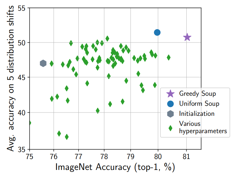
The method described above is the simplest one, called uniform soup. A method called greedy soup uses a validation dataset: you sort models by validation performance and add them to the soup one by one. Initially, the soup contains only the best validation model. You then consider adding models in descending validation performance order, and compute the validation performance of the averaged parameters of the current soup. If performance improves, you keep the addition; if it worsens, you revert and do not add that model. After processing all models, you take the average of the models that remained in the soup as the final model. Greedy soup requires a validation dataset and is slightly more complex, but it has been confirmed to outperform uniform soup (see the model-soup performance figure above).

Stochastic weight averaging (SWA; Izmailov+ 2018) is also a method that improves performance by averaging parameters, similarly to model soup. In SWA, after training, you run stochastic gradient descent with a sufficiently large learning rate for some time, obtain a trajectory of parameters \(\boldsymbol{\theta}_1, \boldsymbol{\theta}_2, \ldots, \boldsymbol{\theta}_n \in \mathbb{R}^d\), and average them. It can be viewed as an easy-to-make model soup produced from a single training run.

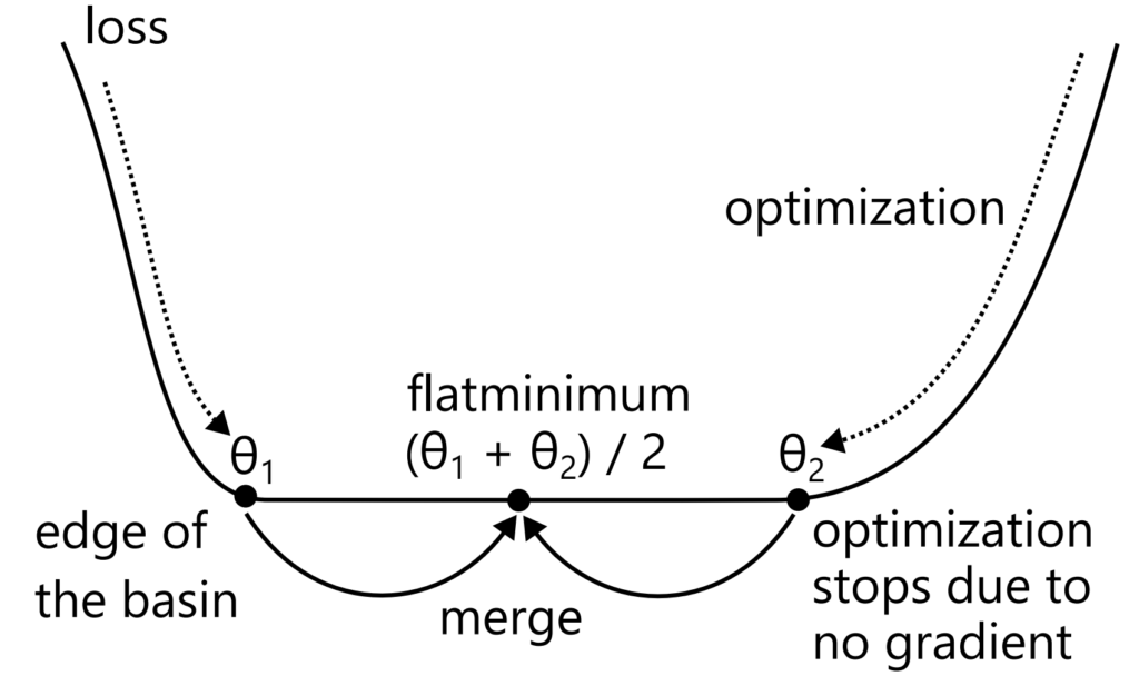
Why does model soup achieve higher performance than a single model? There are several explanations. First, model soup tends to land in flat minima (see the flat-minima figure below). Parameters obtained by fine-tuning from the same pretrained model are linearly mode connected and belong to the same basin. Within a basin, the loss function is convex, so by Jensen’s inequality, averaging reduces the loss. More precisely, the loss can remain the same, but it does not increase. Even if averaging does not reduce the loss, it tends to produce a flatter solution located more centrally within the basin. When optimizing with gradient methods, training stops once the loss reaches 0. If the basin is wide (as in the flat-minima figure), this means training may stop at the edge of the basin. Even among solutions with the same training loss 0, flatter solutions are expected to generalize better. This has also been experimentally confirmed.

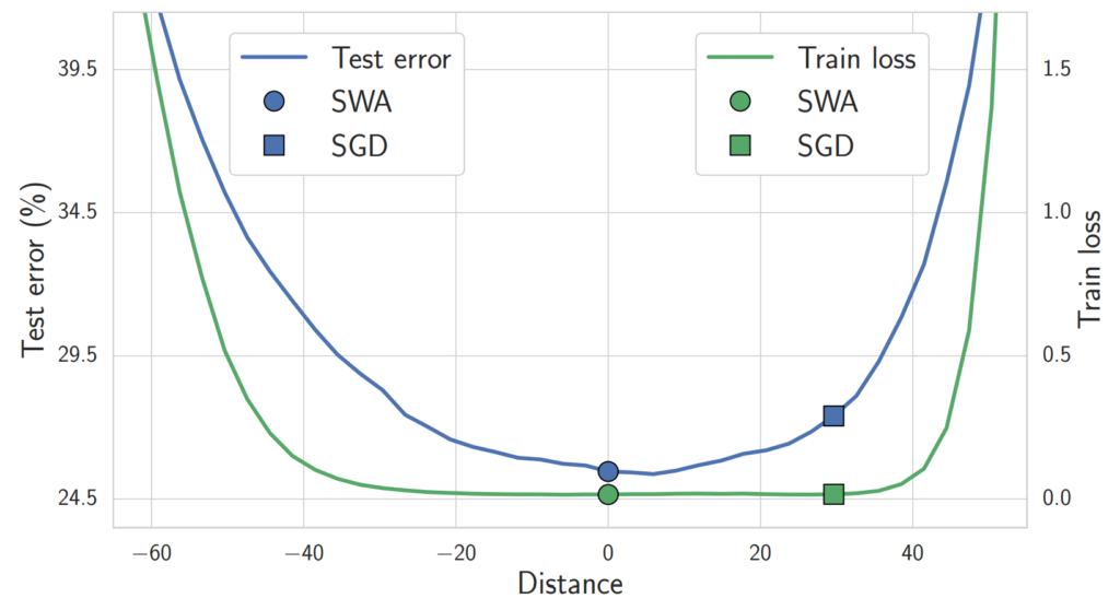
The loss-interpolation figure below plots training error and test misclassification rate for parameters \(\boldsymbol{\theta}^*\) (the final parameters trained by SGD on CIFAR-100 with VGG-16) and \(\boldsymbol{\theta}_{\text{SWA}}\) (parameters obtained by SWA), along the interpolation \(\boldsymbol{\theta} = \alpha \boldsymbol{\theta}^* + (1 – \alpha) \boldsymbol{\theta}_{\text{SWA}}\). The training error is similarly low for both, but the SGD solution \(\boldsymbol{\theta}^*\) lies at the edge of the basin, while the SWA solution \(\boldsymbol{\theta}_{\text{SWA}}\) lies near the center. The test misclassification rate is smaller closer to the center of the basin, and \(\boldsymbol{\theta}_{\text{SWA}}\) has better generalization performance than \(\boldsymbol{\theta}^*\).

Second, model soup can be viewed as an approximation to an ensemble. Let \(f(\cdot; \boldsymbol{\theta})\) be the function represented by the model. An ensemble averages in function space:

\[
f_{\text{ens}}(x) = \frac{1}{n} \sum_{i = 1}^n f(x; \boldsymbol{\theta}_i).
\]

Now expand \(f\) in \(\boldsymbol{\theta}\) around \(\boldsymbol{\theta} = \boldsymbol{\theta}_{\text{unif}}\) using a Taylor expansion:

\[
f(x; \boldsymbol{\theta}_i) = f(x; \boldsymbol{\theta}_{\text{unif}}) + (\boldsymbol{\theta}_i – \boldsymbol{\theta}_{\text{unif}})^\top \nabla_{\boldsymbol{\theta}} f(x; \boldsymbol{\theta}_{\text{unif}}) + O(|\boldsymbol{\theta}_i – \boldsymbol{\theta}_{\text{unif}}|^2).
\]

Substitute this into the ensemble expression:

\[
f_{\text{ens}}(x) – f(x; \boldsymbol{\theta}_{\text{unif}}) = \frac{1}{n} \sum_{i = 1}^n (\boldsymbol{\theta}_i – \boldsymbol{\theta}_{\text{unif}})^\top \nabla_{\boldsymbol{\theta}} f(x; \boldsymbol{\theta}_{\text{unif}}) + O(|\boldsymbol{\theta}_i – \boldsymbol{\theta}{\text{unif}}|^2).
\]

Note that by the definition of \(\boldsymbol{\theta}_{\text{unif}}\),

\[
\frac{1}{n} \sum_{i = 1}^n (\boldsymbol{\theta}_i – \boldsymbol{\theta}_{\text{unif}}) = 0.
\]

Therefore, the difference between model soup and the ensemble becomes

\[
f_{\text{ens}}(x) – f(x; \boldsymbol{\theta}_{\text{unif}}) = \frac{1}{n} \sum_{i = 1}^n O(|\boldsymbol{\theta}_i – \boldsymbol{\theta}_{\text{unif}}|^2).
\]

In other words, the difference is second order or smaller. When fine-tuning from a pretrained model, parameter changes are small, so \(\|\boldsymbol{\theta}_i – \boldsymbol{\theta}_{\text{unif}}\|\) is also small, and the uniform model soup and the ensemble are close as functions. As mentioned above, an ensemble increases inference computation time by a factor of \(n\) and complicates deployment, while a uniform model soup can achieve a similar effect with a single model.

Merging LoRA

In practice, merging LoRA is often performed. In particular, for generative AI such as Stable Diffusion, it is common for end users to distribute LoRA models they trained themselves on the web. Other users often download multiple LoRA modules and apply several LoRA modules at once. Since LoRA is trained as an addition to the original model, applying multiple LoRA modules should not work well in principle, but in practice it often works even without special tricks. This can be explained by the fact that LoRA is also a kind of fine-tuning: the difference from the original model is small, so merging works for the reasons described above.

Merging Models Without Alignment

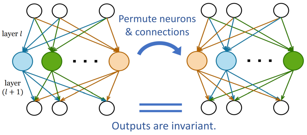
Note that all models added to a model soup are fine-tuned from the same pretrained model. In general, if you average models trained from different random initializations, you do not obtain a good model. Intuitively, with different random initializations the dimensions are not aligned, so simple averaging destroys structure. More concretely, the permutation invariance of neural networks plays an important role [Entezari+ 2022]. Neurons in a neural network can be permuted without changing the model’s functional behavior (see the permutation-invariance figure below). However, this permutation swaps parameter dimensions, producing a completely different parameter vector. Models trained from different random initializations do not share the same permutation, so averaging mixes mismatched dimensions, producing a meaningless result.

Conversely, even for unaligned models, if we can permute neurons to align them properly, we should be able to merge them. Entezari et al. (2022) proposed the hypothesis that models obtained by SGD from different initializations can be made linearly mode connected by an appropriate neuron permutation, and they obtained experimental results supporting this. Somepalli et al. (2022) found that models trained by SGD from different initializations can differ substantially as parameter vectors, yet have similar decision boundaries. These results suggest that models trained from different initializations still use essentially similar inference mechanisms, so if we can align them, merging should be possible.

In Entezari et al.’s experiments, the alignment was found by a simple search using simulated annealing. Methods have since been proposed that compute more effective permutations and enable merging of models trained from different random initializations, or even models with different architectures.

Git Re-Basin [Ainsworth+ 2023] aligns unaligned models by computing appropriate neuron permutations. The input is two models A and B that have the same architecture, number of layers, and width, but differ in initialization and/or training procedure. The output is a single model with the same architecture as the inputs. The goal is to obtain a model that generalizes better than either input, or a model that combines what the two input models learned.

Git Re-Basin proposes three alignment methods. The first uses activation matrices. Consider aligning neuron permutations in a specific layer (for example, layer 1). Suppose this layer has \(d\) neurons, and for \(n\) data points, let \(\boldsymbol{Z}_A \in \mathbb{R}^{d \times n}\) and \(\boldsymbol{Z}_B \in \mathbb{R}^{d \times n}\) be the matrices whose columns (or arranged entries) are the \(d\)-dimensional activations of models A and B. This method solves a matching problem using \(\boldsymbol{C} = \boldsymbol{Z}_A \boldsymbol{Z}_B^\top \in \mathbb{R}^{d \times d}\) as the score matrix. Here \(\boldsymbol{Z}_{A,i} \in \mathbb{R}^n\) represents the firing pattern of neuron \(i\) over the \(n\) data points, and \(\boldsymbol{C}_{ij} = \boldsymbol{Z}_{A,i}^\top \boldsymbol{Z}_{B,j}\) is the inner-product similarity between the firing patterns of neuron \(i\) in model A and neuron \(j\) in model B. Higher similarity indicates the neurons represent the same information, so we permute neurons to make such pairs correspond. This is performed for all layers.

The second alignment method uses weight matrices. Let \(\boldsymbol{W}_A \in \mathbb{R}^{d_l \times d_{l+1}}\) and \(\boldsymbol{W}_B \in \mathbb{R}^{d_l \times d_{l+1}}\) be parameter matrices of models A and B. The method finds a permutation of the rows of \(\boldsymbol{W}_A\) that makes it close to \(\boldsymbol{W}_B\) in Euclidean distance. However, permuting the rows of layer \(l\) affects the columns of layer \(l-1\), so layers cannot be solved independently. Git Re-Basin therefore uses a block coordinate descent style procedure: it computes permutations for each layer in sequence and repeats across all layers until convergence. Compared with activation-based alignment, weight-based alignment has the advantage that it does not require input data.

The third method treats the permutation of model B’s neurons as parameters and optimizes the permutation to maximize the performance of the merged model obtained by merging A and permuted B. Because permutation operations are non-differentiable, the method uses the straight-through estimator (STE) for optimization. This method requires input data and includes parameter optimization, so it is the most computationally expensive, but it achieves the best performance among the three methods. The three methods represent a trade-off between computation and performance, and you can choose depending on your situation.

Optimal transport fusion [Singh+ 2020] can be applied to models with different widths. It is similar in spirit to activation-based or weight-based alignment described above, but it uses optimal transport to compute a soft matching, making it applicable even when widths are not identical.

Evolutionary model merge [Akiba+ 2024] can be applied to merging models from different domains or with different architectures. In general, for models with different numbers of layers or different structures, it uses evolutionary computation to optimize which layers to merge with which layers, in what order, and by which merge method. The objective is performance on a target task. The merged model typically has a different number of layers and a different architecture from the original models. For example, the first layer might be a merge of layer 1 of model A and layer 1 of model B; the second layer might merge layer 2 of A with layer 3 of B; the third layer might reuse layer 4 of A as-is; and so on. Why it works even when you merge layers from different architectures or reorder layers is not fully understood, but skip connections are one plausible reason.

A model with skip connections updates intermediate representations sequentially as

\[
\boldsymbol{x}_{l+1} = \boldsymbol{x}_l + f_l(\boldsymbol{x}_l; \boldsymbol{\theta}_l).
\]

If you slightly change the order of these updates, the final result may not change much. In experiments by Veit et al. (2016), removing a layer from a model without skip connections caused a severe performance drop, while for models with skip connections, performance was preserved to some extent even after removing some layers. They also confirmed that for models with skip connections, changing the order in which layers are applied does not significantly change performance. In experiments by Liu et al. (2023), for large language models the norm of the update \(f(\boldsymbol{x}_l; \boldsymbol{\theta}_l)\) is extremely small compared to the norm of the input/output, and intermediate representations change smoothly. In particular, consecutive representations \(\boldsymbol{x}_l\) and \(\boldsymbol{x}_{l+1}\) are very close. In that case,

\[
\begin{aligned}
\boldsymbol{x}_{l+1} &= \boldsymbol{x}_l + f_l(\boldsymbol{x}_l; \boldsymbol{\theta}_l) \\ \boldsymbol{x}_{l+2} &= \boldsymbol{x}_{l+1} + f_{l+1}(\boldsymbol{x}_{l+1}; \boldsymbol{\theta}_{l+1}) \\
&\approx \boldsymbol{x}_l + f_l(\boldsymbol{x}_l; \boldsymbol{\theta}_l) + f_{l+1}(\boldsymbol{x}_l; \boldsymbol{\theta}_{l+1})
\end{aligned}
\]

and similarly, even if we swap the order,

\[
\begin{aligned}
\boldsymbol{x}’_{l+1} &= \boldsymbol{x}_l + f_{l+1}(\boldsymbol{x}_l; \boldsymbol{\theta}_{l+1}) \\
\boldsymbol{x}’_{l+2} &= \boldsymbol{x}’_{l+1} + f_l(\boldsymbol{x}’_{l+1}; \boldsymbol{\theta}_l) \\ &\approx \boldsymbol{x}_l + f_l(\boldsymbol{x}_l; \boldsymbol{\theta}_l) + f_{l+1}(\boldsymbol{x}_l; \boldsymbol{\theta}_{l+1})
\end{aligned}
\]

the result does not change much. In this view, each layer \(f(\boldsymbol{x}_l; \boldsymbol{\theta}_l)\) can be seen as a small independent model that produces an update, and layer \(l\) does not necessarily need to be placed in position \(l\). Merging different layers from different architectures can be understood as searching over how to apply these updates.

Task Vectors

Task vectors [Ilharco+ 2023] are vectors that represent the learning of a task. Learning and unlearning can be realized via arithmetic on task vectors.

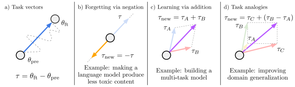
Start from a pretrained model \(\boldsymbol{\theta}_0 \in \mathbb{R}^d\). If \(\boldsymbol{\theta}_1\) is the result of fine-tuning on the dataset of task A, then \(\boldsymbol{\tau}_A = \boldsymbol{\theta}_1 – \boldsymbol{\theta}_0\) is called the task vector for task A.

It is known that learning and unlearning can be achieved by task vector arithmetic. For example, a model with parameters \(\boldsymbol{\theta}_0 + \boldsymbol{\tau}_A + \boldsymbol{\tau}_B\) achieves high performance on both tasks A and B. It has been confirmed, for instance, that if you add a task vector for solving math problems to a dialogue model, it becomes a dialogue model with strong math ability [Yu+ 2023]. Also, let the pretrained model be a language model, and let task C be “insulting language”. If you train on a text corpus consisting of insults to obtain task vector \(\boldsymbol{\tau}_C\), then the language model with parameters \(\boldsymbol{\theta}_0 – \boldsymbol{\tau}_C\) does not produce insults.

Interestingly, task vectors can perform analogical reasoning similar to word vectors. For word vectors, it is known that king – man + woman \(\approx\) queen. Something similar can be done with task vectors. For example, let task A be language modeling on Amazon reviews, task B be language modeling on Yelp reviews, and task C be sentiment analysis on Amazon reviews. Then the model with parameters \(\boldsymbol{\theta}_0 + \boldsymbol{\tau}_C + (\boldsymbol{\tau}_B – \boldsymbol{\tau}_A)\) achieves good performance on sentiment analysis for Yelp reviews. As another example, let task A be a dataset of dog photos, task B be a dataset of lion photos, and task C be a dataset of dog illustrations. Then the model with parameters \(\boldsymbol{\theta}_0 + \boldsymbol{\tau}_C + (\boldsymbol{\tau}_B – \boldsymbol{\tau}_A)\) can correctly classify lion illustrations. In this way, even if you have none or only a small amount of data for the desired task, you can solve it by arithmetic on task vectors constructed from datasets in other domains.

Model Parameters and the Neural Tangent Kernel

Model-parameter arithmetic becomes easier to understand through the neural tangent kernel (NTK) [Ortiz-Jimenez+ 2023].

Let the pretrained model parameters be \(\boldsymbol{\theta}_0 \in \mathbb{R}^d\). The neural tangent kernel \(k\) defined by this model is

\[
\begin{aligned}
k(x, x’) &\stackrel{\text{def}}{=} \phi(x)^\top \phi(x’) \
\phi(x) &\stackrel{\text{def}}{=} \nabla_{\boldsymbol{\theta}} f(x; \boldsymbol{\theta}_0) \in \mathbb{R}^d.
\end{aligned}
\]

This can be interpreted as using \(\phi(x)\) as a feature vector and measuring similarity by an inner product. Two data points \(x\) and \(x’\) with a large neural tangent kernel value can be regarded as similar in terms of how they influence updates to model \(\boldsymbol{\theta}_0\). The term “tangent” refers to tangents and tangent planes: the gradient \(\phi(x) = \nabla_{\boldsymbol{\theta}} f(x; \boldsymbol{\theta})\) represents a tangent plane, which motivates the name.

Perform fine-tuning using stochastic gradient descent (SGD) and update parameters as

\[
\boldsymbol{\theta}_{i + 1} = \boldsymbol{\theta}_i + \alpha_i \nabla_{\boldsymbol{\theta}} f(x_i; \boldsymbol{\theta}_i).
\]

Here \(\alpha_i \in \mathbb{R}\) is the product of the learning rate and the gradient of the loss with respect to the function output, \(\frac{\partial \ell}{\partial f}\). Without loss of generality, we assume the output of \(f\) is one-dimensional. The learning rate is a small positive value, and the sign of \(\frac{\partial \ell}{\partial f}\) depends on the loss. If the output should be increased for that training sample, \(\alpha_i\) is positive; if the output should be decreased, \(\alpha_i\) is negative. Suppose fine-tuning produces parameters \(\boldsymbol{\theta}_n\).

Assume parameters did not move much during training, and take a first-order Taylor approximation around \(\boldsymbol{\theta} = \boldsymbol{\theta}_0\). Then the function represented by \(\boldsymbol{\theta}_n\) can be written as

\[
\begin{aligned}
f(x; \boldsymbol{\theta}_n) &\approx f(x; \boldsymbol{\theta}_0) + (\boldsymbol{\theta}_n – \boldsymbol{\theta}_0)^\top \nabla_{\boldsymbol{\theta}} f(x; \boldsymbol{\theta}_0) \\
&= f(x; \boldsymbol{\theta}_0) + (\boldsymbol{\theta}_n – \boldsymbol{\theta}_0)^\top \phi(x).
\end{aligned}
\]

That is, the difference from the pretrained model can be seen as a linear model that uses the NTK feature map \(\phi(x)\) as a feature extractor.

If we expand the history of parameter updates, we obtain

\[
\begin{aligned}
f(x; \boldsymbol{\theta}_n) &\approx f(x; \boldsymbol{\theta}_0) + (\boldsymbol{\theta}_n – \boldsymbol{\theta}_0)^\top \nabla_{\boldsymbol{\theta}} f(x; \boldsymbol{\theta}_0) \\ &= f(x; \boldsymbol{\theta}_0) + (\boldsymbol{\theta}_n – \boldsymbol{\theta}_0)^\top \phi(x) \\ &= f(x; \boldsymbol{\theta}_0) + \left(\sum_{i = 0}^{n – 1} \boldsymbol{\theta}_{i + 1} – \boldsymbol{\theta}_i \right)^\top \phi(x) \\ &= f(x; \boldsymbol{\theta}_0) + \left(\sum_{i = 0}^{n – 1} \alpha_i \nabla_{\boldsymbol{\theta}} f(x_i; \boldsymbol{\theta}_i) \right)^\top \phi(x) \\ &\stackrel{\text{(a)}}{\approx} f(x; \boldsymbol{\theta}_0) + \left(\sum_{i = 0}^{n – 1} \alpha_i \phi(x_i) \right)^\top \phi(x) \\
&= f(x; \boldsymbol{\theta}_0) + \sum_{i = 0}^{n – 1} \alpha_i k(x_i, x).
\end{aligned}
\]

In (a) we used the approximation \(f(x_i; \boldsymbol{\theta}_i) \approx f(x_i; \boldsymbol{\theta}_0)\). For a test data point that is not similar to any training data \(x_i\), the kernel values in the second term are zero, so the output equals the pretrained model output. If a test point is similar to a training sample \(x_i\), then the term \(\alpha_i k(x_i, x) \approx (\boldsymbol{\theta}_{i + 1} – \boldsymbol{\theta}_i)^\top \phi(x)\) becomes non-zero, and the output becomes the pretrained model output plus the learned contribution from that training sample. If the test point is similar to multiple training samples, all their learned contributions accumulate. Recall that \(\alpha_i\) is positive if the output should be increased for that training sample, and negative if the output should be decreased. If the output should be increased for a similar training sample \(x_i\), then \(\alpha_i k(x_i, x)\) is positive; if it should be decreased, then \(\alpha_i k(x_i, x)\) is negative. The fine-tuned model output is the cumulative effect of these terms.

Rather than focusing on a specific test sample \(x\), consider the difference between the function represented at initialization and after training:

\[
f(x; \boldsymbol{\theta}_n) – f(x; \boldsymbol{\theta}_0) \approx \sum_{i = 0}^{n – 1} \alpha_i k(x_i, x).
\]

Define

\[
f_{\text{diff}}(x) \stackrel{\text{def}}{=} \sum_{i = 0}^{n – 1} \alpha_i k(x_i, x).
\]

It is helpful to view this as a function representation by Parzen windows (see the Parzen-window figure below). Each training data point influences its neighborhood through a Parzen window \(k(x_i, x)\).

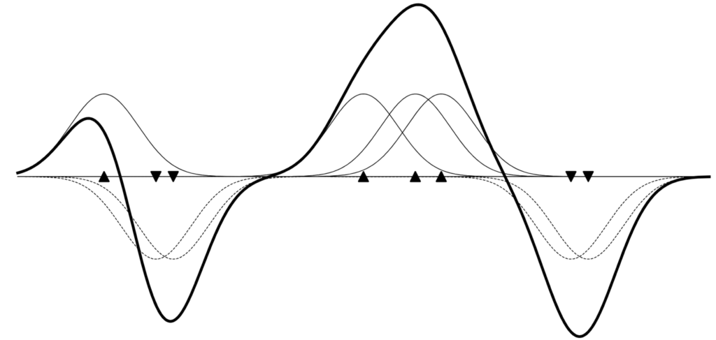
At this point, the relationship among (1) training data, (2) model parameters, and (3) the function represented by the model becomes clear. Training data affects model parameters through the term \((\boldsymbol{\theta}_{i + 1} – \boldsymbol{\theta}_i) \approx \alpha_i \phi(x_i)\). This corresponds to adding the NTK feature vector \(\phi(x_i)\) of that sample into the model parameters, scaled by how the function value should change. From the function viewpoint, this corresponds to shifting values up or down using Parzen windows \(\alpha_i k(x_i, x)\).

Model parameters \(\boldsymbol{\theta}_A\) trained on the dataset \(D_A\) of task A have accumulated the NTK feature vectors of the training data in \(D_A\). The task vector for task A is a weighted sum of NTK feature vectors.

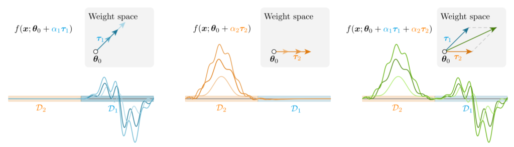
The sum of the task vector for task A and the task vector for task B corresponds to adding the union of NTK feature vectors from the datasets of task A and task B. This gives an intuitive explanation for why learning happens via the sum of task vectors (see the NTK task-vector figure above).

Model soup can also be interpreted as adding NTK feature vectors to a soup. Since the training data is the same, this does not fully explain the mechanism, but intuitively, different hyperparameters add features at slightly different angles, which can make similarity measurement more robust.

Conclusion

Model merging is a magical technique that lets you create the model you want without expensive training.

And the principles behind that magic are increasingly being explained using theory such as the neural tangent kernel.

Try using model merging to easily build the model you want.

Author Profile

If you found this article useful or interesting, I would be delighted if you could share your thoughts on social media.

New posts are announced on @joisino_en (Twitter), so please be sure to follow!