Interestingness First Classifiers

Most existing machine learning models aim to maximize predictive accuracy, but in this article, I will introduce classifiers that prioritize interestingness.

What Does It Mean to Prioritize Interestingness?

For example, let us consider the task of classifying whether a user is an adult based on their profile.
If the profile contains an age feature, then the rule “age ≥ 18” would achieve 100% accuracy. On social media, there is always a possibility that users write down a false age, but in most cases people report their age more or less correctly, so this rule would likely achieve around 99% accuracy. The accuracy of this classification rule is extremely high, but it is not interesting.

Let us consider a more unusual rule: “if the registered email address ends with @icloud.com then the user is a minor, whereas the user is an adult if it ends with @aol.com.” Such a rule might achieve a reasonable level of accuracy. Even though the accuracy would not be particularly high, it is interesting—and that makes it valuable. This is the kind of classifier we want to obtain.

As a more academic example, consider the problem of detecting depressive symptoms. Various tests have been proposed for this purpose. One famous example is the Beck Depression Inventory, which asks respondents to rate themselves on 21 items such as whether they feel depressed, whether they are pessimistic about the future, or whether they feel guilty. Each item is answered on a four-point scale, and the total score is used to make a judgment. This test is widely used for diagnosing depression, but whether the judgment rule is “interesting” is questionable. Being told, “You are strongly pessimistic about the future, therefore you are depressed,” is not exactly surprising.

Other, more interesting results have also been reported. For example, it is known that one can achieve a certain level of accuracy by having people write an essay and then checking whether they frequently use first-person words (I, my, me, myself). If such words occur more often, the person is more likely to be depressed [Rude+ 2004, Edwards+ 2017]. The idea is that people with depressive tendencies are more likely to focus on information about themselves rather than about their surroundings or the external world. Of course, this method is heavily influenced by individual writing styles; a cheerful person might also use “I” frequently. In fact, although this judgment method is statistically significant, the correlation coefficient is only about r = 0.13, which is not very high. Even so, because of its interestingness, this rule has gained a certain reputation in psychology, and it has led to a variety of related and follow-up studies [Edwards+ 2017].

For a somewhat more practical example that we will use in this article, let us consider the problem of determining whether someone is present in an office (the Occupancy Detection dataset). For this dataset, a simple rule based on whether the lights are on in the office achieves about 99% accuracy. Offices generally have their lights on even during the day, and in most companies, people do not stay or sleep in the office with the lights off. Thus, the relationship “lights on = someone is present” holds almost perfectly. But if the problem can be solved this way, it is not very interesting.

As we will see later, this problem can actually be solved with about 85% accuracy using the rule “if humidity is high, then someone is present.” Of course, if the humidity is high, one cannot distinguish whether it is due to rain or to the presence of people, and even if people are present, humidity may not rise very much, so the accuracy cannot be extremely high. Still, the idea that the presence of people can be inferred with a hygrometer is intriguing: it feels like it could work, or maybe it couldn’t, which makes it sit at just the right level of interestingness. Moreover, beyond being simply “interesting” or not, if such a non-obvious sensor can solve the problem, it suggests the possibility of implementing applications that do not require very high accuracy at lower cost than before. In this sense, it also has practical value.

Related topics include feature selection, model interpretability, and explainability, but these are fundamentally different from prioritizing interestingness because they primarily aim to maximize accuracy. For instance, if one applies feature selection to the adult classification problem, the feature “age” would be chosen, leading to the interpretable rule “age ≥ 18.” This rule is interpretable and highly accurate, but not interesting. Likewise, for the problem of determining whether someone is present in an office, the feature “light” would be selected, giving the rule “light ≥ 300.” This, too, is interpretable and highly accurate, but not interesting.

Problem Setting

The input is tabular data. We assume something like a Pandas DataFrame, where the first d columns are features and the final column is the label to be predicted.

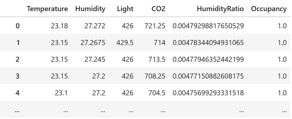
The goal is to automatically obtain classification rules that are interesting or unexpected. This is the same setup as the typical classification problem often seen in Kaggle: table in, classifier out. However, whereas conventional approaches aim to maximize predictive accuracy, here we prioritize interestingness, while still seeking to achieve a meaningful level of accuracy.

Method

The proposed method, EUREKA (Exploring Unexpected Rules for Expanding Knowledge boundAries), is very simple. Put briefly, it uses an LLM to select interesting features and then builds a classifier using only those interesting features.

The selection of interesting features works as follows: we ask the LLM, “Suppose you could predict X using only feature A, and likewise you could predict X using only feature B. Which one would be more interesting?” This is repeated across multiple pairs of features to construct a ranking of interestingness. The ranking is formed by ordering features according to how many times they were chosen. Despite its simplicity, this approach is known to be nearly optimal [Shah+ JMLR 2018].

For example, when applied to the task of classifying whether someone is present in an office (the Occupancy Detection dataset), this produces the following ranking of features:

1. HumidityRatio (the ratio of water vapor mass in the air to the mass of dry air)
2. Humidity
3. Temperature
4. Light
5. CO₂

It would be interesting if we could determine whether an office is occupied using only humidity, whereas determining it from CO₂ is trivial.

There is a subtle trick in asking the LLM to choose between two features at a time. If we instead asked it to “rate how interesting each feature is,” the scoring criteria would shift each time, and features might be selected just because they happened to receive a lenient score. Moreover, many LLMs are biased toward giving positive responses, so if we asked them to rate on a ten-point scale, the responses would cluster near the top (close to 10), producing many ties. Pairwise comparison, by contrast, relies on relative rather than absolute judgments, so it avoids problems of shifting baselines. Forcing the choice of “which one is more interesting” ensures that the evaluation does not end in universal ties, and small differences between candidates are reflected. Another appealing point is that this method can be used even when only a black-box API is available.

Once we have the ranking of interesting features, we then train classifiers using only the top K interesting features (e.g., K = 1 feature, K = 3 features, etc.). For instance, we might test whether the presence of people in an office can be determined using only HumidityRatio, or using only HumidityRatio, Humidity, and Temperature. The classifier can be any interpretable model, such as logistic regression or decision trees. In the following, we use logistic regression.

Experimental Results

First, let us apply both conventional feature selection methods and the proposed method to various datasets to see which features are selected as the most important. For the proposed method, it can happen that a feature with no predictive power at all is ranked first; in such cases, we also list the second-ranked feature. (With conventional methods, this never occurs, since they always prioritize features with higher predictive power. This happens precisely because the proposed method prioritizes interestingness over predictive power.)

Dataset	Task	Group LASSO	Logistic Regression	Validation Selection	EUREKA (ours)
Occupancy Detection	Predict whether a room is occupied	Light	Light	Light	HumidityRatio, Humidity
Twin Papers	Predict which paper is cited more	Lengthen_the_reference if the reference list is longer	Lengthen_the_reference if the reference list is longer	Lengthen_the_reference if the reference list is longer	Including_a_Colon_in_the_Title
Mammographic Mass	Predict benign vs. malignant mass	BI-RADS score assigned by radiologist	BI-RADS score assigned by radiologist	BI-RADS score assigned by radiologist	Density, Age mass density and patient age
Breast Cancer Wisconsin	Predict benign vs. malignant tumor	Bare_nuclei frequency of exposed nuclei	Bare_nuclei frequency of exposed nuclei	Uniformity_of_cell_size	Marginal_adhesion cell-to-cell adhesion strength
Adult	Predict if income > $50k	capital-gain	capital-gain	capital-gain	capital-loss
Website Phishing	Predict if a site is phishing	SFH (Server Form Handler)	SFH (Server Form Handler)	SFH (Server Form Handler)	popUpWindow

Conventional methods—though differing in criteria—all aim to select features that are useful for prediction, and thus tend to choose similar features. By contrast, the proposed method produces feature selections that look quite different.

As mentioned earlier, in the Occupancy Detection dataset (predicting whether someone is in a room), the most predictive feature is illumination, but the most interesting feature turns out to be humidity.

In the Twin Papers dataset (predicting which of two similar papers will be more cited), the strongest predictive feature is “length of references.” Indeed, longer reference lists suggest that the work is well-researched and firmly grounded in prior studies, which makes it more likely to be high-quality and hence cited. Moreover, in the modern citation ecosystem, citing another paper increases its exposure (e.g., backlinks on Google Scholar pages), which further raises the chance of it being cited.

However, prioritizing interestingness yields the feature “whether the title contains a colon.” This is a rather eccentric feature, but as we will see later, this feature alone provides a meaningful signal about citation counts.

In the Mammographic Mass dataset (predicting malignancy of breast tumors), BI-RADS is a manual score assigned by radiologists. Since it comes from expert diagnosis, it is extremely reliable. Using it for prediction yields very high accuracy, so it is often excluded from prediction competitions. Here, however, we deliberately included it. As expected, existing feature selection methods identify BI-RADS as the most predictive feature. The proposed method, on the other hand, does not prioritize BI-RADS—since that would not be interesting—but instead highlights other features such as density and age.

In the Adult dataset (predicting whether annual income is above $50k), conventional methods choose capital-gain, while the proposed method chooses capital-loss. Indeed, income can also be predicted from losses, and doing so feels more interesting than focusing on gains.

When logistic regression is trained using capital-loss, the result is: “the larger the losses, the higher the probability that income ≥ $50k.” This achieves a respectable level of accuracy. The finding that greater losses correspond to higher income is somewhat counterintuitive, but makes sense: individuals with income < $50k often lack assets to sell, so they are unlikely to incur large capital losses. Substantial capital losses are more likely to occur from real estate transactions or similar, implying that the individual owns significant assets. Thus, many losses → high income. That is interesting.

The accuracy of classifiers trained using features selected by the proposed method is as follows:

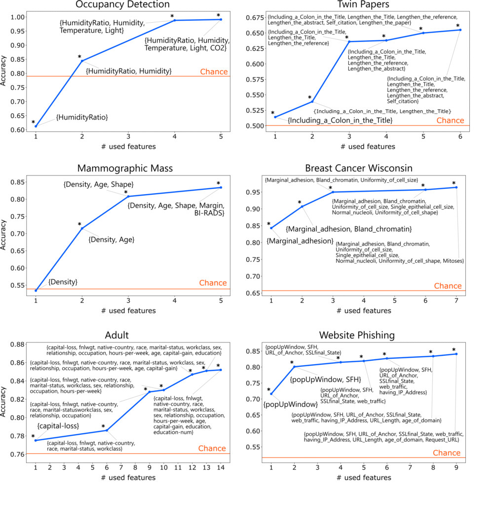
In most cases, even when only the single most interesting feature is used, accuracy exceeds the chance rate (the accuracy obtained by always predicting the majority class). The exceptions are the HumidityRatio feature in the Occupancy Detection dataset and the Density feature in the Mammographic Mass dataset. Although HumidityRatio alone shows a statistically significant fit, the effect size is small and class imbalance prevents it from surpassing the chance rate in terms of accuracy. Even in such cases, including the second-most interesting feature raises accuracy above the chance rate.

As described earlier, in the Occupancy Detection dataset, the rule “high humidity → someone present” achieves about 85% accuracy.

In the Twin Papers dataset, the rule “titles containing a colon are more likely to be cited” achieves about 52% accuracy. For example, papers like “Twin Papers: A Simple Framework of Causal Inference for Citations via Coupling” or “Beyond Exponential Graph: Communication-Efficient Topologies for Decentralized Learning via Finite-time Convergence” fall into this category. Including a concise concept or method name before the colon makes the title more eye-catching and memorable. While the accuracy seems low, the test set contains as many as 17,000 instances, so an improvement of about 2% over the chance rate represents a statistically powerful signal. The finding “titles with colons receive (slightly) more citations” is much less obvious—and more interesting—than “papers with many citations tend to be cited more.”

Interestingly, the feature judged least interesting is Self_citation (whether the author cites their own past work). Of course, it is obvious that self-citing increases citation counts. Indeed, trained classifiers confirm that self-citation has a strong positive effect on the number of citations.

The key point here is that such interesting rules can automatically emerge simply by feeding in tabular data.

Finally, let us touch on spurious correlations. As with conventional classifiers, the rules produced by this approach may reflect spurious correlations. If necessary, one could proceed to causal analysis from here. However, under the doctrine of interestingness-first, spurious correlations are not a major concern. For example, there is a famous spurious rule: “In years when Nicolas Cage appeared in many films, more people drowned by falling into swimming pools” [Vigen 2015].

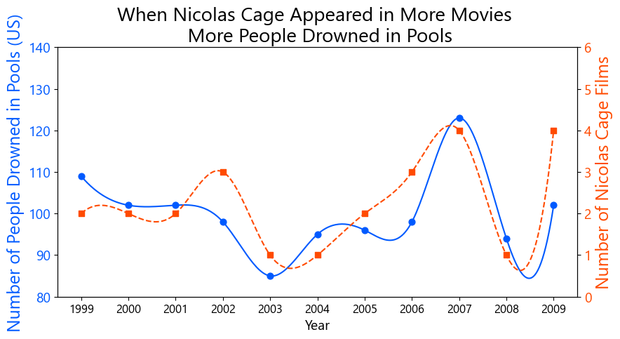
Of course, this is pure coincidence, but it is so amusing that it has been widely cited and used in textbooks on statistics and causal inference. Discovering such entertaining spurious correlations is, in terms of interestingness, valuable in its own right. Naturally, one must be careful not to confuse correlation with causation, and should certainly avoid misguided actions like drowning many people in pools just to watch more Nicolas Cage’s films.

Conclusion

It is certainly satisfying when a classifier achieves high accuracy, but it is also delightful when we obtain classifiers that are interesting. In competitions like Kaggle, performance is usually judged by accuracy, but I think it would be nice if there were also contests where people competed on interestingness.

I hope this article serves as a trigger for paying attention not only to classifier accuracy but also to their interestingness.

arXiv: Interesting First Classifiers

Author Profile

If you found this article useful or interesting, I would be delighted if you could share your thoughts on social media.

New posts are announced on @joisino_en (Twitter), so please be sure to follow!