What I like about this result is that it combines a strong “wait, you can do that?” feeling with real research usefulness. I recently used it in our paper, and since ChatGPT could not answer it when I asked, I decided to write this post. The original source is Dynamic Generation of Discrete Random Variate.
Problem setting
Suppose we are given a sequence of length \( N \),
\( w_1, w_2, \ldots, w_N \in \mathbb{R}_+ \).
You can think of the weight \( w_i \) as something like the importance of element \( i \).
We would like to sample from \( 1, 2, \ldots, N \) with probability proportional to these weights.
We would also like to be able to change the values of the sequence along the way.
That is, we want to answer the following two kinds of queries:
- Sampling: sample from the discrete distribution
\[
\frac{w_1}{\sum_i w_i}, \frac{w_2}{\sum_i w_i}, \ldots, \frac{w_N}{\sum_i w_i}
\] - Update: given \( (i, x) \), update \( w_i \leftarrow x \)
These queries may arrive in any order and in arbitrary number, and we aim to process each query in expected constant time even in the worst case. Here, “expected time” means expectation over the internal randomness of the randomized algorithm; we do not assume any distribution over the query sequence. We also aim to keep the preprocessing time at \( O(N) \) and the memory usage at \( O(N) \).
A naive implementation would process each query in \( \Theta(N) \) time. If you have done competitive programming, you can probably think of a way to process each query in \( \Theta(\log N) \) time. Getting this down to \( O(1) \) is quite nontrivial.
This kind of problem appears often in machine learning and data processing, especially in online learning. The sequence plays the role of parameters; each time data arrives, we update the parameters, and when making a prediction, we sample from them. For example, in our paper, we used this in the computational complexity analysis of Exp3, an algorithm for the multi-armed bandit problem. It is a fairly general problem setting, and the result is strong, so it may be worth remembering as a trick you can pull out when needed.
Below, let \( W = \sum_i w_i \) denote the total weight. This value may change under updates, but we maintain it explicitly and update it in constant time whenever an update happens.
For readers interested in a deeper formulation: when discussing running time, the assumptions on the computational model matter. Here we assume a random access machine. That is, each \( w_i \) and \( N \) fits in one machine word, and basic operations such as arithmetic, logarithms, ceilings, and memory access on them can be done in constant time. We assume the word size is large enough to hold \( W = \sum_i w_i \). We also assume that we can sample a uniform random number from \( [0, 1] \) in constant time. Without such assumptions, on a bare Turing machine, even outputting “\( N \)” already takes \( O(\log N) \) time, so discussing constant-time algorithms would not make sense. This is why the assumption is necessary. On real computers, this assumption is approximately satisfied by representing \( w_i \) and \( N \) using float, int64, and so on.
1. The case without updates (the alias method)
When there are no updates, there is a very famous method called the alias method.
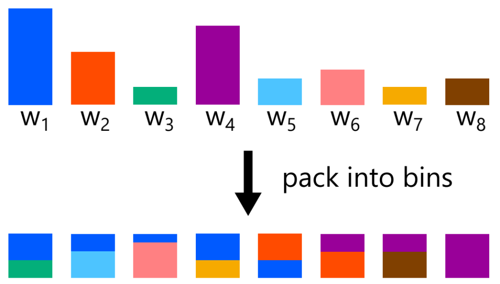
The alias method packs the weights \( w_1, w_2, \ldots, w_N \) into \( N \) boxes in a clever way. If done properly, each box contains at most two colors. When sampling, we first choose a box uniformly from \( 1, 2, \ldots, N \). Suppose the weights inside the chosen box are \( a \) and \( b \). We then sample \( r \sim \mathrm{Unif}(0, a + b) \), and output the first color if \( r < a \), and the other color otherwise. This gives constant-time sampling from the weights \( w_1, w_2, \ldots, w_N \).
The following procedure yields a packing in which each box contains at most two colors.
- Let \( \bar{W} = \frac{W}{N} \) be the target weight per box.
- Put each weight \( w_i \) into the small group if \( w_i < \bar{W} \), and into the large group if \( w_i \ge \bar{W} \).
- Take one weight from the small group and one from the large group. Put the small-group weight into a box, then fill the remaining space in that box with as much of the large-group weight as possible. By the definition of the small group, the small-group weight fits completely into the box; by the definition of the large group, the large-group weight is enough to fill the rest of the box.
- Put the remaining part of the large-group weight back into either the small group or the large group depending on its new size.
- Return to step 3.
There is one exception: if all remaining weights are exactly \( \bar{W} \), then we simply place them one by one into boxes. Otherwise, there must always be both weights smaller than \( \bar{W} \) and weights larger than \( \bar{W} \), so step 3 can continue.
The alias method is easy to implement and very fast in practice, so it is well suited to the case without updates. However, it does not handle updates well.
Next, let us look at a method that does support updates, but uses far too much memory.
2. A brute-force approach (prefix sums and lookup tables)
When the weights are integers
Here let the length of the sequence be \( n \), and suppose \( w_1, w_2, \ldots, w_n \) are positive integers with maximum value \( m = \max_i w_i. \)
Prepare an array of length \( W = w_1 + w_2 + \cdots + w_n, \) and color positions \( 1 \) through \( w_1 \) with color \( 1 \), positions \( w_1 + 1 \) through \( w_1 + w_2 \) with color \( 2 \), and so on, so that color \( i \) occupies \( w_i \) consecutive positions. This gives a lookup table.
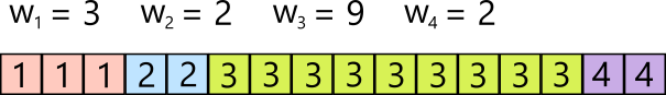
To sample, we draw \( i \) uniformly from \( 1, 2, \ldots, W \), and output the value stored in position \( i \) of the lookup table. This gives constant-time sampling.
When the weights are real numbers
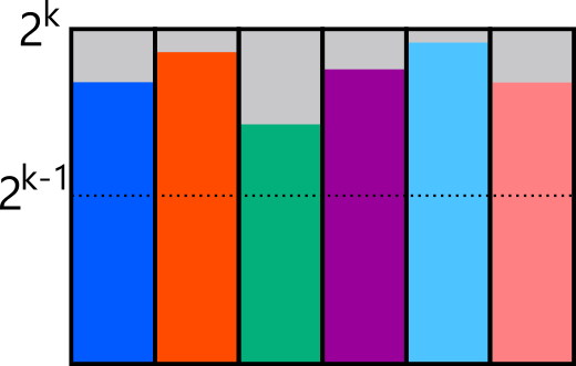
Now suppose the weights \( w_1, w_2, \ldots, w_n \) are real numbers at least \( 1 \). If some weights are at most \( 1 \), we can normalize appropriately so that this assumption holds.
In this case, we first round each \( w_i \) up to an integer, and then apply the method above.
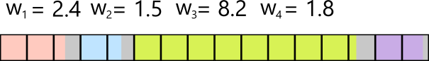
Of course, rounding up to integers slightly distorts the distribution.
To correct this, we use rejection sampling. If index \( i \) is sampled under the rounded-up distribution, we accept it with probability \( \frac{w_i}{\lceil w_i \rceil}, \) and otherwise reject it and sample again. In the figure above, this corresponds to resampling whenever we hit the gray region. Since \( w_i \ge 1 \), the acceptance probability is at least \( \frac{1}{2} \), so the expected number of trials until acceptance is at most \( 2 = O(1). \)
When updates are allowed
Let us now adapt the integer-weight data structure to support updates.
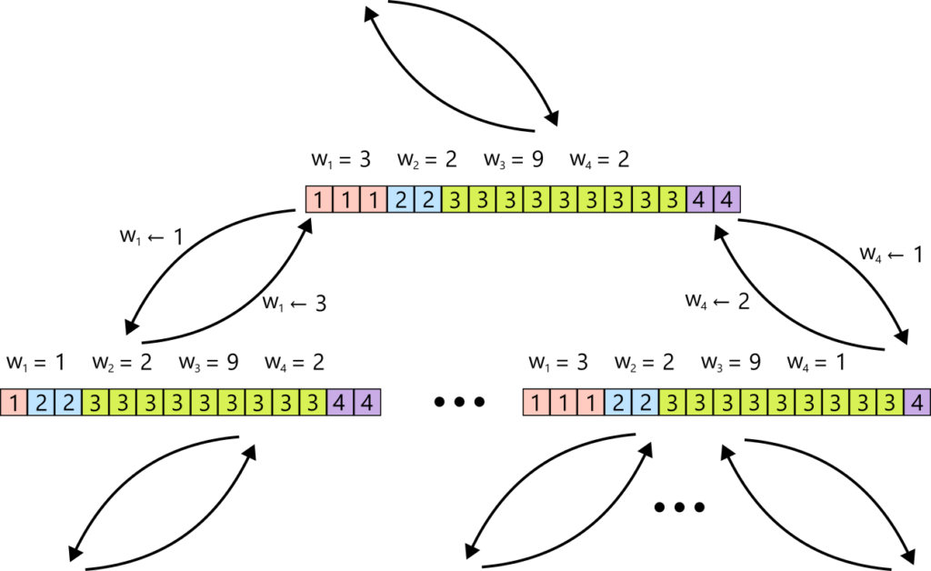
The idea is completely brute-force. A positive sequence of length \( n \) with maximum value \( m \) has only \( m^n \) possibilities. So we precompute a lookup table for every possible sequence, and for each such sequence, we also record, for every possible update operation, which lookup table we should move to next. Then, when an update \( (i, x) \) arrives, we simply switch to the corresponding next lookup table, and sampling is done in constant time using that table.
Thus we have achieved expected constant-time sampling and updates.
The problem, of course, is the preprocessing time and the memory usage.
We need, for all \( m^n \) possible positive sequences, a lookup table of length \( O(nm) \), and for each of the \( O(nm) \) possible update operations, a pointer to the next table. Therefore the total space and preprocessing time become \( O(n m^{n+1}). \)
We wanted linear-time preprocessing, but this is exponential. So this is not practical.
3. Constant-time sampling and updates for discrete distributions
Now we finally move to the general case.
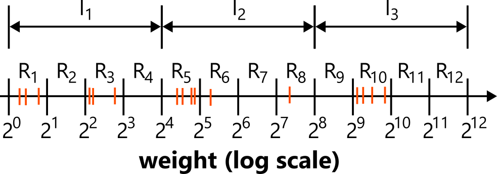
Split the positive line of weights into ranges
\[
R_1 = [1, 2), \quad R_2 = [2, 4), \quad R_3 = [4, 8), \ldots
\]
that is,
\[
R_k = [2^{k-1}, 2^k).
\]
Assign each weight \( w_i \) to its corresponding range. For each range, we keep the list of assigned weights and also the total weight in that range, denoted \( W_{R_k} \).
Next, group the ranges into intervals of size \( \lceil \log N \rceil \):
- \( I_1 = (R_1, R_2, \ldots, R_{\lceil \log N \rceil}) \)
- \( I_2 = (R_{\lceil \log N \rceil + 1}, R_{\lceil \log N \rceil + 2}, \ldots, R_{2 \lceil \log N \rceil}) \)
- and so on.
Each interval stores the list of ranges it contains and the sum of their weights.
Using ranges and intervals, we can naively sample as follows.
- Choose an interval with probability proportional to its weight.
- Within the chosen interval, choose a range with probability proportional to its weight.
- Within the chosen range, choose an element with probability proportional to its weight.
However, the number of intervals, the number of ranges in an interval, and the number of elements in a range are not constant, so this alone does not give constant time.
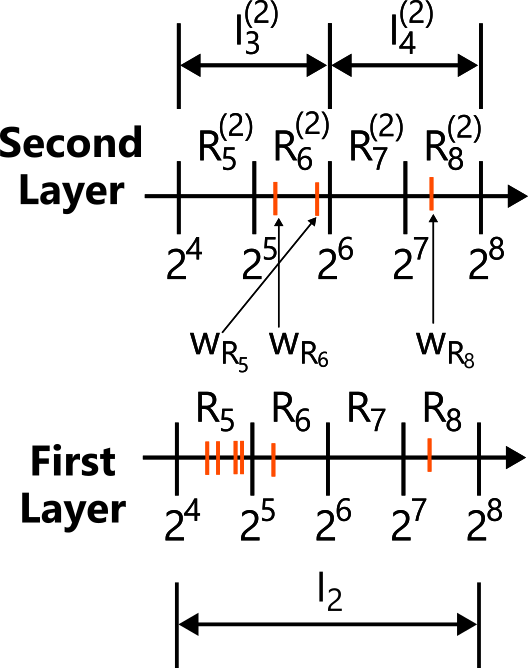
Step 2, “choose a range within the chosen interval with probability proportional to its weight,” has exactly the same structure as the original problem. So for each interval, we introduce the same structure one level deeper using the range weights.
At first glance this may look like just adding another layer, but it makes the second-level size extremely small, and then the brute-force approach from Section 2 becomes applicable.
First, a first-level interval contains at most \( \lceil \log N \rceil = O(\log N) \) ranges. These now play the role of \( N \) when building the second level, so each second-level interval \( I_j^{(2)} \) contains at most
\[
\lceil \log \lceil \log N \rceil \rceil = O(\log \log N)
\]
ranges \( R_k^{(2)} \).
Moreover, after normalization, the maximum possible weight becomes
\[
2 \cdot \lceil \log N \rceil^2 = O(\log^2 N),
\]
as can be shown.
Range \( R_k^{(2)} \) inside second-level interval \( I_j^{(2)} \) contains at most \( \lceil \log N \rceil \) values of the form \( W_{R_\ell} \), and each of those weights lies in the interval
\[
[2^{(j – 1)\lceil \log \lceil \log N \rceil \rceil},\ 2^{j \lceil \log \lceil \log N \rceil \rceil}).
\]
So if at least one such weight is assigned to \( R_k^{(2)} \), then
\[
2^{(j – 1)\lceil \log \lceil \log N \rceil \rceil}
\le
W_{R_k^{(2)}}
<
\lceil \log N \rceil \cdot 2^{j \lceil \log \lceil \log N \rceil \rceil}.
\]
Now divide by \( 2^{(j – 1)\lceil \log \lceil \log N \rceil \rceil} \) and define the normalized weight \( W’_{R_k^{(2)}} \). Then \[ 1 \le W'{R_k^{(2)}} < \lceil \log N \rceil \cdot 2^{\lceil \log \lceil \log N \rceil \rceil}.
\]
Hence
\[
1 \le W’_{R_k^{(2)}} < \lceil \log N \rceil \cdot 2^{1 + \log \lceil \log N \rceil} = 2 \cdot \lceil \log N \rceil^2.
\]
The brute-force method from Section 2 runs in \( O(n m^{n+1}) \). If we apply it with
\[
n = \lceil \log \lceil \log N \rceil \rceil,
\qquad
m = 2 \cdot \lceil \log N \rceil^2,
\]
then the preprocessing time and memory usage become
\[
O(n m^{n+1}) = o(N),
\]
that is, asymptotically smaller than linear.
First,
\[
\frac{n m^{n+1}}{N}
=
\frac{
\lceil \log \lceil \log N \rceil \rceil
\cdot
\left( 2 \cdot \lceil \log N \rceil^2 \right)^{\lceil \log \lceil \log N \rceil \rceil + 1}
}{N}.
\]
Equivalently,
\[
\frac{n m^{n+1}}{N}
=
2^{
\log \lceil \log \lceil \log N \rceil \rceil
+
\left( \log \left( 2 \cdot \lceil \log N \rceil^2 \right) \right)
\left( \lceil \log \lceil \log N \rceil \rceil + 1 \right)
–
\log N
}.
\]
Now look at the exponent. The first term is of order \( O(\log \log \log N) \), the second term is polynomial in \( \log \log N \), and the third term is of order \( O(\log N) \). The third term is exponentially larger than the others, so as \( N \to \infty \),
\[
\frac{n m^{n+1}}{N} \to 0.
\]
Thus at this tiny size, the brute-force method indeed runs in \\( O(n m^{n+1}) = o(N) \\).
So if we precompute this transition structure of lookup tables for that \( (n, m) \), then every second-level interval can share the same structure, and within each second-level interval, both sampling and updates can be done in constant time.
Therefore we can sample as follows:
- Among all first-level intervals, choose a first-level interval with probability proportional to its weight.
- Within the chosen first-level interval, choose a second-level interval with probability proportional to its weight.
- Within the chosen second-level interval, sample a second-level range with probability proportional to its weight using the brute-force method from Section 2.
- Within the chosen second-level range, choose a first-level range with probability proportional to its weight.
- Within the chosen first-level range, choose an element with probability proportional to its weight.
This makes step 3 constant time.
We have passed the main hurdle, but we still need to speed up the other steps.
For step 1, we stop trying to sample from all candidates directly.
Let
\[
t = \left\lceil \frac{\lceil \log W \rceil}{\lceil \log N \rceil} \right\rceil.
\]
The maximum element is on the order of \( W = \sum w_i \), so we expect it to lie in a range around \( \log W \), and hence in an interval around \( t \). Strictly speaking, we would like to use \( \max w_i \), but computing \( \max w_i \) cannot be done in constant time. So instead we use the rough but constant-time proxy \( W \).
Since interval weights decrease exponentially as we move left, intervals other than \( I_t, I_{t-1}, I_{t-2}, I_{t-3} \) contribute almost nothing to the total probability.
So we do the following:
- Compute
\[
t = \left\lceil \frac{\lceil \log W \rceil}{\lceil \log N \rceil} \right\rceil.
\] - Look at intervals \( I_t, I_{t-1}, I_{t-2}, I_{t-3} \), and obtain their total weights \( W_t, W_{t-1}, W_{t-2}, W_{t-3} \).
- Let
\[
W^- = W – W_t – W_{t-1} – W_{t-2} – W_{t-3}.
\] - Sample one of
\[
(W_t, W_{t-1}, W_{t-2}, W_{t-3}, W^-)
\]
with probability proportional to its weight. - If one of the first four choices is selected, then we have selected an interval. If the last choice is selected, only then do we spend \( O(N) \) time to sample directly.
It can be shown that this is valid. First, the maximum element lies in an interval around \( t \), so at least one of \( W_t \) and \( W_{t-1} \) is nonzero.
Since
\[
\max w_i < \sum_i w_i \le N \max w_i,
\]
if the range containing \( \max w_i \) is \( k \), then
\[
2^{k-1} \le \max w_i < W \le N \max w_i \le N 2^k.
\]
Taking logarithms,
\[
k – 1 < \log W \le k + \log N.
\]
Hence
\[
k – 1 < \lceil \log W \rceil \le k + \lceil \log N \rceil,
\]
so
\[
k \le \lceil \log W \rceil \le k + \lceil \log N \rceil,
\]
and therefore
\[
\lceil \log W \rceil – \lceil \log N \rceil \le k \le \lceil \log W \rceil.
\]
The interval containing range \( k \) is
\[
j = \left\lceil \frac{k}{\lceil \log N \rceil} \right\rceil,
\]
so
\[
\left\lceil \frac{\lceil \log W \rceil}{\lceil \log N \rceil} \right\rceil – 1
\le
j
\le
\left\lceil \frac{\lceil \log W \rceil}{\lceil \log N \rceil} \right\rceil.
\]
Next, we can show that
\[
\frac{W^-}{W} \le \frac{1}{N}.
\]
Let \( j \) be the interval containing \( \max w_i \). Since \( j \ge t – 1 \),
\[
W = \sum_i w_i \ge \max w_i \ge 2^{(j – 1)\lceil \log N \rceil} \ge 2^{(t – 2)\lceil \log N \rceil}.
\]
Every weight \( w_i \) that belongs to an interval indexed at most \( t – 4 \) satisfies
\[
w_i \le 2^{(t – 4)\lceil \log N \rceil}.
\]
There are at most \( N \) such weights contributing to \( W^- \), so
\[
W^- \le N \cdot 2^{(t – 4)\lceil \log N \rceil}.
\]
Therefore,
\[
\frac{W^-}{W} \le \frac{N \cdot 2^{(t-4)}\lceil \log N \rceil}{2^{(t-2)}\lceil \log N \rceil} = N \cdot 2^{-2 \lceil \log N \rceil} \le N \cdot 2^{-2 \log N} = \frac{1}{N}
\]
So the probability that \( W^- \) is chosen is at most \( \frac{1}{N} \). Even if we spend \( O(N) \) time only in that case, the expected running time remains constant.
Step 2 has the same structure, so the same trick gives expected constant time there as well.
For steps 4 and 5, we use rejection sampling, exploiting the fact that the weights within a given range are all nearly the same.
A range is \( R_k = [2^{k-1}, 2^k). \) Prepare one box of size \( 2^k \) for each element in the range, and place one element in each box. First choose a box uniformly. If the chosen box corresponds to element \( \ell \) with weight \( w_\ell \), then sample \( r \sim \mathrm{Unif}(0, 2^k), \) and accept this element if \( r < w_\ell \); otherwise reject and sample again. Since every box is at least half full, the expected number of trials until acceptance is at most \( 2 = O(1). \)
This completes constant-time sampling.
Updates are also easy because the structure was designed for them. Suppose we update \( w_i \leftarrow x \). We subtract the old \( w_i \) from the total weights of the corresponding first-level and second-level intervals and ranges, move the second-level interval to the appropriate next lookup-table state, then add the new \( w_i \) to the corresponding first-level and second-level intervals and ranges, and again move the second-level interval to the appropriate next state. This gives constant-time updates as well.
Strictly speaking, one has to be careful about how the elements are stored. Given an index \( i \), we must be able to access “the \( i \)-th interval” or “the \( i \)-th range” in constant time. If we simply store pointers in an array, then access is constant time, but when the range of possible weights is extremely large, the nonempty intervals and ranges may be very sparse, and we would need an enormous array. Then the memory usage would no longer necessarily be \( O(N) \). So instead, if the number of nonempty intervals (or ranges) is \( K \), we store them in a hash table of size \( \Theta(K) \). With a bad hash function, lookup could take linear time in the worst case, but with universal hashing, lookup takes expected constant time. This ensures that memory usage is proportional only to the number of nonempty objects, so the total memory remains \( O(N) \). The same applies to the boxes used for rejection sampling inside a range, which can likewise be maintained so that insertions and deletions take constant time. Of course, the number of elements inside an interval or range can change. In that case, when the table becomes full, we rebuild it at twice the size, and when it becomes only one-quarter full, we rebuild it at half the size. This keeps the size always at \( \Theta(K) \), and since we spend \( O(K) \) time on rebuilding only once every \( \Theta(K) \) operations, the running time is amortized constant.
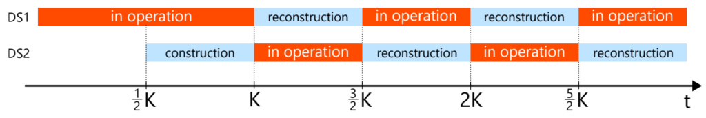
Moreover, if we maintain two copies of this data structure, then while one is being rebuilt, the other can continue to serve requests. In this way, we can even obtain worst-case constant time. If rebuilding finishes in \( cK \) steps, then each time the currently active table handles a request, we spend \( 2c \) background steps advancing the rebuild. Then each request still takes constant time, and the rebuild completes within \( K/2 \) rounds.
Variants and related remarks
Up to this point, we have done rather complicated things to force constant time, but this comes with a few drawbacks from a practical point of view.
First, using the brute-force method from Section 2 inside each second-level interval is attractive if one wants literal constant time, but in practice the constant factor is large, so it is not very practical. In practice, it is often better to process the second-level interval naively, or to add one more layer and process that last layer naively, which reduces the constant-factor overhead.
Second, I described the step where we sample from
\[
(W_t, W_{t-1}, W_{t-2}, W_{t-3}, W^-),
\]
but when the fifth choice is selected, one suddenly pays a large computational cost. This happens rarely, but it is still inconvenient. In the original paper, they propose a more practical variant with slightly worse theoretical complexity but smaller variance in the running time. That variant uses the same idea of partitioning into ranges, but does not use intervals; instead, it recursively groups ranges into larger ranges and samples through that recursive structure.
The method introduced here is very general. In special cases, one can implement something simpler and more efficient. For example, in our paper, we considered the case where each update does not completely replace the weights by unrelated new values, but instead changes them only slightly from the previous ones. In that case, we showed that a slight modification of the alias method already solves the same problem in expected constant time. And the Exp3 algorithm for the multi-armed bandit problem indeed satisfies this condition, so we showed that it can be implemented efficiently. This version is very simple: even in Python, it takes only about 20 lines on top of the alias method. The paper also includes code, so please take a look if you are interested. In machine learning and data analysis applications, cases where the weights change only a little from one step to the next, rather than becoming completely unrelated new values, seem quite common.
Closing
I really like the “wait, you can do that?” feeling of this result. I found the problem setting mysterious the first time I heard it, I found the method mysterious the first time I understood it, and even now, after spending more than ten thousand Japanese characters writing this explanation, it still feels mysterious.
I think the key points are that sampling, unlike many other computational problems, can tolerate constant-factor slack because rejection sampling lets us recover an exact algorithm, and that the power of the random access machine model is being pushed to the limit here, especially its somewhat unusual ability to compute logarithms in constant time.
Will there ever come a day when this result feels obvious to me? Until that day, I will keep studying.
Author Profile
If you found this article useful or interesting, I would be delighted if you could share your thoughts on social media.
New posts are announced on @joisino_en (Twitter), so please be sure to follow!

Ryoma Sato
Currently an Assistant Professor at the National Institute of Informatics, Japan.
Research Interest: Machine Learning and Data Mining.
Ph.D (Kyoto University).