TwoNN Intrinsic Dimension Explained: Python and Visual Illustrations

Real-world data often live in a high-dimensional ambient space, but the points themselves concentrate near a much lower-dimensional manifold. The “visible” (ambient) dimension is easy to read off from the feature vector length, while the “intrinsic” dimension (the effective degrees of freedom) is much harder to estimate.

Two Nearest Neighbors (TwoNN) is a simple yet surprisingly effective estimator of intrinsic dimension. It uses only the first and second nearest-neighbor distances at each data point, and fits a straight line after a log transform.

The TwoNN Algorithm

Given a dataset of \(N\) points \(\{x_i\}_{i=1}^N\):

1. For each point \(x_i\), compute:

• \(r_{1,i}\): the distance to its nearest neighbor
• \(r_{2,i}\): the distance to its second nearest neighbor
  Then define the ratio
  \[
  \mu_i = \frac{r_{2,i}}{r_{1,i}}.
  \]

1. Sort the ratios in ascending order:
   \[
   \mu_{(0)} \le \mu_{(1)} \le \cdots \le \mu_{(N-1)}.
   \]
2. Create points
   \[
   \left(\ln \mu_{(k)},\; -\ln\left(1 – \frac{k}{N}\right)\right), \quad k=0,1,\ldots,N-1.
   \]
3. Fit a straight line through the origin by least squares:
   \[
   d = \frac{x^\top y}{x^\top x},
   \]
   where \(x_k = \ln \mu_{(k)}\) and \(y_k = -\ln\left(1 – \frac{k}{N}\right)\).
   The slope \(d\) is the estimated intrinsic dimension.

Intuitive Derivation (Why the Line Appears)

Fix a point \(x\). Let \(x_1\) be its nearest neighbor and \(x_2\) its second nearest neighbor.

Consider the ball centered at \(x\) with radius \(r_2\). By definition, there is exactly one neighbor (\(x_1\)) inside this ball closer than \(r_2\), and the next one (\(x_2\)) lies on its boundary at distance \(r_2\).

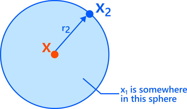
Now assume \(r_2\) is small enough that the density around \(x\) is approximately constant (a “locally uniform” approximation). Under this approximation, the location of \(x_1\) is roughly uniform inside the radius-\(r_2\) ball.

Consider the outer ball centered at \(x\) with radius \(r_2\). Now look at the “inner” ball with half the radius, \(r_2/2\).

• If \(x_1\) lies exactly on the boundary of the inner ball, then \(r_1 = r_2/2\), so
  \[
  \mu = \frac{r_2}{r_1} = \frac{r_2}{r_2/2} = 2.
  \]
• If \(x_1\) lies inside the inner ball, then \(r_1 < r_2/2\), so \(\mu > 2\).
• If \(x_1\) lies outside the inner ball (but still inside the outer ball), then \(r_1 > r_2/2\), so \(\mu < 2\).

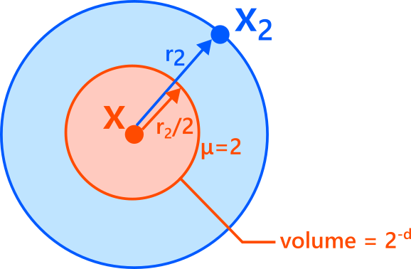
Assuming the density is approximately constant within the outer ball, the probability that \(x_1\) falls inside the inner ball is proportional to the ratio of volumes. If the intrinsic dimension is \(d\), volume scales as radius\(^d\), hence
\[
P(\mu \ge 2)
= P\left(r_1 \le \frac{r_2}{2}\right)
\approx \frac{\mathrm{Vol}(\text{ball of radius } r_2/2)}{\mathrm{Vol}(\text{ball of radius } r_2)}
= \left(\frac{1}{2}\right)^d
= 2^{-d}.
\]

Similarly, consider the inner ball with one-third the radius, \(r_2/3\).

• If \(x_1\) lies exactly on its boundary, then \(r_1 = r_2/3\), so \(\mu = 3\).
• If \(x_1\) lies inside this ball, then \(r_1 < r_2/3\), so \(\mu > 3\).
• If \(x_1\) lies outside it, then \(r_1 > r_2/3\), so \(\mu < 3\).

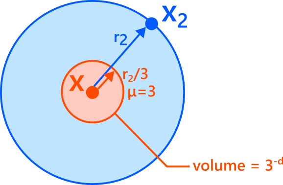
Again by volume scaling,
\[
P(\mu \ge 3)
= P\left(r_1 \le \frac{r_2}{3}\right)
\approx \left(\frac{1}{3}\right)^d
= 3^{-d}.
\]

More generally, for any \(a > 1\), consider the inner ball of radius \(r_2/a\). Then
\[
P(\mu \ge a)
= P\left(r_1 \le \frac{r_2}{a}\right)
\approx \left(\frac{1}{a}\right)^d
= a^{-d}.
\]

This is the tail probability of \(\mu\). Therefore, the cumulative distribution function is
\[
F(\mu) = P(\mu’ \le \mu) \approx 1 – \mu^{-d}
\quad (\mu \ge 1).
\]

From the Distribution to a Linear Fit

If we sort observed ratios \(\mu_{(k)}\), then \(\mu_{(k)}\) approximately corresponds to the empirical quantile \(k/N\), so:
\[
\frac{k}{N} \approx F\left(\mu_{(k)}\right)
= 1 – \mu_{(k)}^{-d}.
\]
Rearrange:
\[
1 – \frac{k}{N} \approx \mu_{(k)}^{-d}.
\]
Take logs:
\[
-\ln\left(1 – \frac{k}{N}\right) \approx d \ln \mu_{(k)}.
\]
So if we plot \(y_k = -\ln\left(1 – \frac{k}{N}\right)\) against \(x_k = \ln \mu_{(k)}\), the points should lie near a straight line through the origin with slope \(d\).

That is exactly what TwoNN fits.

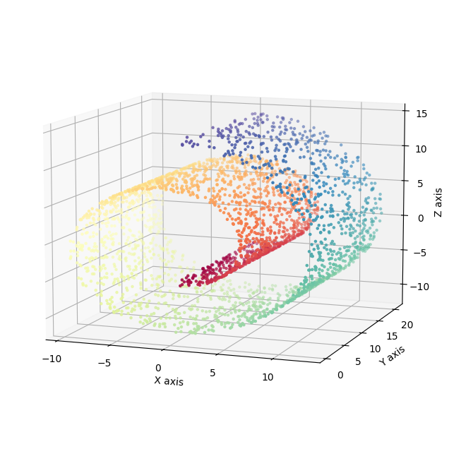
Numerical Example: Swiss Roll

Swiss Roll is a classic example: it is a two-dimensional manifold embedded in three dimensions.

Below is a minimal Python implementation you can paste into your environment.

import numpy as np
import matplotlib.pyplot as plt
from sklearn.datasets import make_swiss_roll
from sklearn.neighbors import NearestNeighbors

def two_nn_intrinsic_dimension(X, plot_fit=True):
    """
    Estimates the Intrinsic Dimension (ID) of a dataset using the TWO-NN algorithm.

    Args:
        X (numpy.ndarray): Input data array of shape (n_samples, n_features).
        plot_fit (bool): If True, plots the linear regression fit.

    Returns:
        float: The estimated intrinsic dimension.
    """
    
    N = X.shape[0]
    
    # ---------------------------------------------------------
    # Step 1: Compute pairwise distances and find 
    # the first two nearest neighbors.
    # ---------------------------------------------------------
    # We need k=3 because the 1st neighbor is the point itself (distance 0).
    # So, index 1 is the 1st NN, index 2 is the 2nd NN.
    nbrs = NearestNeighbors(n_neighbors=3, algorithm='auto').fit(X)
    distances, indices = nbrs.kneighbors(X)

    # Extract r1 (1st neighbor dist) and r2 (2nd neighbor dist)
    # distances[:, 0] is the distance to self (0.0)
    r1 = distances[:, 1]
    r2 = distances[:, 2]
    mu = r2 / r1
    
    # ---------------------------------------------------------
    # Step 2: Compute the empirical Cumulate Distribution Function (CDF).
    # ---------------------------------------------------------
    # Sort mu values in ascending order.
    mu_sorted = np.sort(mu)
    
    # The empirical CDF F(mu_i) is defined as i / N.
    F_emp = np.arange(N) / N
    
    # ---------------------------------------------------------
    # Step 3: Linear Regression to find the dimension d.
    # The theory states: -log(1 - F(mu)) = d * log(mu)
    # ---------------------------------------------------------
    # X axis: log(mu)
    x = np.log(mu_sorted)
    
    # Y axis: -log(1 - F(mu))
    y = -np.log(1 - F_emp)
    
    # Perform Linear Regression passing through the origin.
    # Model: y = slope * x
    # The closed-form solution for slope (d) minimizing sum of squared errors
    # for a line through origin is: sum(x*y) / sum(x^2).
    slope = np.dot(x, y) / np.dot(x, x)
    intrinsic_dim = slope
    
    # ---------------------------------------------------------
    # Optional: Visualization of the fit
    # ---------------------------------------------------------
    if plot_fit:
        plt.figure(figsize=(8, 6))
        
        # Plot all points (grey for discarded ones)
        plt.scatter(x, y, s=5, color='#005aff', label='Data points')
        
        # Plot the fitted line
        # Create a line from origin to max x used
        line_x = np.linspace(0, np.max(x), 100)
        line_y = slope * line_x
        plt.plot(line_x, line_y, color='#ff4b00', linewidth=2, label=f'Fit (Slope = ID = {slope:.2f})')
        
        plt.xlabel('ln($\mu$)', fontsize=20)
        plt.ylabel('-ln(1 - F($\mu$))', fontsize=20)
        plt.title(f'TWO-NN Intrinsic Dimension Estimation\nEstimated ID: {intrinsic_dim:.4f}', fontsize=16)
        plt.legend(fontsize=16)
        plt.grid(True, linestyle='--', alpha=0.6)
        plt.show()

    return intrinsic_dim

# =========================================================
# Main Execution
# =========================================================

# 1. Generate Swiss Roll Dataset
# The Swiss Roll is a 2D manifold embedded in 3D space.
# We expect the Intrinsic Dimension (ID) to be approximately 2.
n_samples = 2500

print(f"Generating Swiss Roll dataset with {n_samples} points...")
X, t = make_swiss_roll(n_samples=n_samples, random_state=0)

# 2. Estimate Dimension
print("Running TWO-NN algorithm...")
estimated_d = two_nn_intrinsic_dimension(X, plot_fit=True)

print("-" * 30)
print(f"Ground Truth Dimension : 2.00")
print(f"Estimated Dimension    : {estimated_d:.4f}")
print("-" * 30)

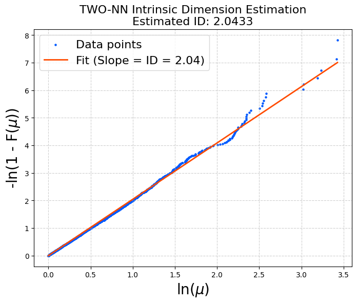
You should see an estimate close to 2.

As often observed, the points deviate more in the large-\(\mu\) region. This is why discarding the top 10% (or similar) before fitting is commonly used.

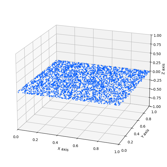
When the Data Contains Noise

If the data has even a small amount of noise off the manifold, then strictly speaking it is no longer exactly low-dimensional. For example, a “thin” manifold with small thickness \(\sigma\) is still a full-dimensional distribution in the ambient space.

If you apply TwoNN to such data, then in the limit of infinite samples the nearest-neighbor distances shrink below the noise thickness, and the estimated dimension will eventually approach the ambient dimension (for a thin board in \(\mathbb{R}^3\), this would approach 3).

However, in practice we often still want to say “the intrinsic dimension is 2” because the meaningful structure is essentially two-dimensional at the scales we care about.

Subsampling as a Scale-Control Trick

A practical workaround is to run TwoNN on random subsamples of different sizes:

• With fewer points, neighbors are farther away (larger \(r_1, r_2\)), so the estimator “sees” the manifold at a coarser scale and is less sensitive to tiny thickness noise.
• With too few points, the estimate becomes unstable and may underestimate the dimension.
• With too many points, neighbors become extremely close and the estimator starts detecting the noise dimension.

So we compute the TwoNN estimate for many subsample sizes \(n\) and look for a plateau region where the estimate stays roughly constant. That plateau value is a good candidate for the “effective” intrinsic dimension at meaningful scales.

Here is an example script.

import numpy as np
import matplotlib.pyplot as plt
from sklearn.neighbors import NearestNeighbors

def two_nn_intrinsic_dimension(X):
    """
    Computes the TWO-NN intrinsic dimension of the dataset X.
    """
    N = X.shape[0]
    nbrs = NearestNeighbors(n_neighbors=3, algorithm='auto', n_jobs=-1).fit(X)
    distances, indices = nbrs.kneighbors(X)
    r1 = distances[:, 1]
    r2 = distances[:, 2]
    mu = r2 / r1
    mu_sorted = np.sort(mu)
    F_emp = np.arange(N) / N
    x = np.log(mu_sorted)
    y = -np.log(1 - F_emp)
    
    # Robustness: Keep only the first 90% of points (discard top 10%)
    n_keep = int(0.9 * N)
    x_fit = x[:n_keep]
    y_fit = y[:n_keep]
  
    slope = np.dot(x_fit, y_fit) / np.dot(x_fit, x_fit)
    
    return slope

def generate_noisy_plane(n_samples, noise_std=0.001):
    """
    Generates points on a unit square in x-y plane with Gaussian noise in z.
    """
    x = np.random.uniform(0, 1, n_samples)
    y = np.random.uniform(0, 1, n_samples)
    z = np.random.normal(0, noise_std, n_samples)
    
    return np.column_stack((x, y, z))


np.random.seed(0)
total_samples = 100000
noise_std = 0.001
n_trials = 100
sample_sizes = [5, 10, 20, 50, 100, 200, 500, 1000, 2000, 5000, 10000, 20000]

print(f"Generating base dataset (N={total_samples}, noise={noise_std})...")
X_full = generate_noisy_plane(total_samples, noise_std)

means = []
stds = []

print("Starting subsampling analysis...")
for n in sample_sizes:
    estimated_ds = []
    for _ in range(n_trials):
        # Subsample randomly
        indices = np.random.choice(total_samples, n, replace=False)
        X_sub = X_full[indices]
        
        # Estimate ID
        d = two_nn_intrinsic_dimension(X_sub)
        estimated_ds.append(d)
    
    # Calculate stats
    mean_d = np.mean(estimated_ds)
    std_d = np.std(estimated_ds)
    means.append(mean_d)
    stds.append(std_d)
    
    print(f"  N={n:4d} : ID = {mean_d:.2f} +/- {std_d:.2f}")

plt.figure(figsize=(10, 6))

# Error bar plot
plt.errorbar(sample_sizes, means, yerr=stds, fmt='o-', capsize=5, 
              color='#005aff', label='Estimated ID (TWO-NN)')

# Reference lines
plt.axhline(y=2.0, color='#03af7a', linestyle='--', linewidth=2, label='True Dimension (Plane = 2)')
plt.axhline(y=3.0, color='#ff4b00', linestyle=':', linewidth=1, label='Embedding Dimension (Space = 3)')

plt.xscale('log')  # Log scale for X axis often makes the trend clearer
plt.xlabel('Sample Size (N) [Log Scale]', fontsize=20)
plt.ylabel('Intrinsic Dimension (d)', fontsize=20)
plt.title(f'Intrinsic Dimension vs Sample Size\n(Noisy Plane, std={noise_std})', fontsize=16)
plt.xticks(sample_sizes, labels=sample_sizes) # Show actual N values on axis
plt.grid(True, which="both", ls="-", alpha=0.4)
plt.legend(fontsize=16)

plt.show()

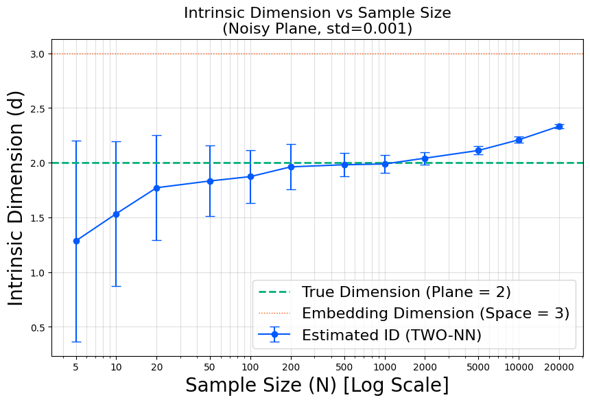
In this specific example, the thin board is a two-dimensional manifold embedded in \(\mathbb{R}^3\), and we add a very small “thickness” noise with \(\sigma = 0.001\). The subsampling plot can be read as follows.

• For subsample sizes \(n \le 50\), TwoNN tends to underestimate the dimension.
• As \(n\) increases, the estimate rises and approaches 2. Around \(n \approx 100\) to \(n \approx 1000\), the curve becomes almost flat: the estimate stays close to 2 over a wide range of \(n\). In this regime, typical neighbor distances are still larger than the noise thickness (larger than about \(10^{-3}\)), so TwoNN mainly “sees” the 2D manifold structure rather than the tiny off-manifold thickness. This plateau is the regime where it makes sense to interpret the intrinsic dimension as approximately 2 for this dataset.
• Once \(n\) exceeds roughly \(1000\), the nearest-neighbor distances become comparable to the noise scale. In this run, the typical \(r_1\) and \(r_2\) values start to fall to around \(10^{-3}\), which is on the order of \(\sigma = 0.001\). From this point on, TwoNN begins to detect the third (thickness) direction, so the estimated dimension starts to drift upward.
• For even larger \(n\), the neighbor distances shrink further below the noise thickness, and the point cloud looks increasingly like a genuinely 3D distribution at that microscopic scale. Consequently, the TwoNN estimate gradually moves toward 3, reflecting the ambient-space dimension \(\mathbb{R}^3\) rather than the underlying 2D manifold.

Summary

TwoNN is a simple and effective method to estimate intrinsic dimension using only nearest-neighbor distance ratios. It works by leveraging a theoretical distribution of \(\mu = r_2/r_1\) under a locally uniform approximation, which turns the estimation problem into a linear regression.

When data contains small off-manifold noise, TwoNN can drift toward the ambient dimension at very large sample sizes. In such cases, subsampling across multiple scales and looking for a plateau often recovers a more meaningful “effective” intrinsic dimension.

Reference

Facco, E., d’Errico, M., Rodriguez, A. et al.
Estimating the intrinsic dimension of datasets by a minimal neighborhood information.
Scientific Reports 7, 12140 (2017).
https://doi.org/10.1038/s41598-017-11873-y

Author Profile

If you found this article useful or interesting, I would be delighted if you could share your thoughts on social media.

New posts are announced on @joisino_en (Twitter), so please be sure to follow!