Fisher Information Explained: Python and Visual Illustrations

Definition of Fisher Information

The Fisher information is defined as

$$
\mathrm{FisherInformation}(\theta_0)
\stackrel{\text{def}}{=}
-\mathbb{E}_{X\sim p(x\mid\theta_0)}
\left[
\frac{d^2}{d\theta^2}\log p(x\mid\theta)\bigg|_{\theta=\theta_0}
\right].
$$

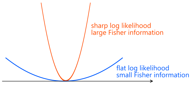
Fisher information quantifies how precisely a model parameter can be estimated.
A larger Fisher information means the parameter can be estimated more accurately,
while a smaller Fisher information indicates that estimation is more difficult.

Fisher information admits several equivalent interpretations.

Equivalent Expressions

$$
\begin{align}
&\mathrm{FisherInformation}(\theta_0) \\
&\stackrel{\text{def}}{=}
-\mathbb{E}_{X \sim p(x \mid \theta_0)}
\left[\frac{d^2}{d\theta^2} \log p(x \mid \theta)\bigg|_{\theta=\theta_0}\right] \\
&\stackrel{\text{(a)}}{\approx}
-\frac{1}{n} \sum_{i = 1}^n
\left[\frac{d^2}{d\theta^2} \log p(x_i \mid \theta)\bigg|_{\theta=\theta_0}\right]
\qquad (x_i \sim p(x \mid \theta_0)\ \text{i.i.d.}) \\
&=
-\frac{d^2}{d\theta^2}
\left(\frac{1}{n} \sum_{i = 1}^n \log p(x_i \mid \theta)\right)\bigg|_{\theta=\theta_0}
\tag{1} \\
&\stackrel{\text{(b)}}{\approx}
-\frac{d^2}{d\theta^2}
\mathbb{E}_{X\sim p(x\mid\theta_0)}[\log p(X\mid\theta)]
\bigg|_{\theta=\theta_0} \\
&=
\frac{d^2}{d\theta^2}
\mathrm{CrossEntropy}(p(x\mid\theta_0), p(x\mid\theta))\bigg|_{\theta=\theta_0} \\
&=
\frac{d^2}{d\theta^2}
\mathrm{KL}(p(x\mid\theta_0),|,p(x\mid\theta))
\bigg|_{\theta=\theta_0}.
\end{align}
$$

Here, (a) and (b) use Monte-Carlo approximation. Under suitable regularity conditions, the equalities hold exactly as \(n\to\infty\).

Thus, Fisher information equals the second derivative (curvature) of the cross-entropy or the Kullback–Leibler divergence with respect to the parameter \(\theta\).
In other words, Fisher information describes the curvature of these functions.
Consequently, when the Fisher information is large, even a small change in \(\theta\) causes the distribution to change significantly, i.e., easy to distinguish.
Conversely, when the Fisher information is small, the distribution remains almost unchanged even if \(\theta\) is perturbed, i.e., difficult to tell apart.

Taylor Expansion of KL Divergence

Let

$$
\mathrm{KL}(\theta)=\mathrm{KL}(p(x\mid\theta_0),|,p(x\mid\theta)).
$$

This function achieves its minimum value \(0\) at \(\theta=\theta_0\).
Therefore, by a Taylor expansion around \(\theta_0\),

$$
\mathrm{KL}(\theta)
\approx
\frac{1}{2}
\mathrm{FisherInformation}(\theta_0)
(\theta-\theta_0)^2.
$$

Thus, Fisher information also appears as the coefficient of the quadratic approximation of the KL divergence.

Numerical Example

We analytically and numerically compute Fisher information for the normal distribution \(\mathcal{N}(0,1)\) with mean \(\mu=0\) and variance \(\sigma^2=1\).

Analytical Calculation

$$
p(x\mid\mu)=\frac{1}{\sqrt{2\pi}}
\exp\left(-\frac{(x-\mu)^2}{2}\right)
$$

$$
\log p(x\mid\mu)
= -\frac12\log(2\pi)-\frac{(x-\mu)^2}{2}
$$

$$
\frac{d^2}{d\mu^2}\log p(x\mid\mu)
= -1
$$

$$\mathrm{FisherInformation}(\mu)=-\mathbb{E}[-1]=1.$$

Numerical Calculation

Using equation (1), we fit a quadratic curve to the average log-likelihood and use its second derivative as a numerical estimate of Fisher information.

import numpy as np
import matplotlib.pyplot as plt

# 1. Generate data from N(0,1)
rng = np.random.default_rng(0)
n = 2000
mu0 = 0.0
sigma = 1.0
x = rng.normal(loc=mu0, scale=sigma, size=n)

# 2. Grid of μ values and mean log-likelihood
mus = np.linspace(-2, 2, 81)

def log_pdf_normal(x, mu, sigma):
    return -0.5 * np.log(2 * np.pi * sigma**2) - 0.5 * (x - mu) ** 2 / (sigma**2)

avg_loglik = np.array([np.mean(log_pdf_normal(x, m, sigma)) for m in mus])

# 3. Quadratic fit
coeffs = np.polyfit(mus, avg_loglik, deg=2)
a, b, c = coeffs
fit_loglik = np.polyval(coeffs, mus)

# 4. Fisher information estimate
fisher_est = -2 * a
print("Estimated Fisher information:", fisher_est)
# => Estimated Fisher information: 1.0000000000000002

# 5. Plot
plt.figure()
plt.plot(mus, avg_loglik, lw=2,
         color="#005aff",
         label="Monte Carlo average log-likelihood")
plt.plot(mus, fit_loglik,
         color="#ff4b00", lw=2,
         linestyle="--",
         label="Quadratic fit")
plt.axvline(mu0, color="gray", linestyle=":", linewidth=1)
plt.xlabel(r"$\mu$", fontsize=16)
plt.ylabel("Average log-likelihood", fontsize=16)
plt.title("Fisher information via quadratic fit", fontsize=16)
plt.legend(fontsize=14)
plt.show()

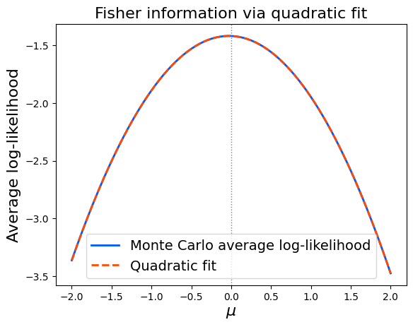
Running the code confirms that the numerical estimate closely matches the analytical value \(1\).

Mixture Model Example

Next, consider a more complex model:

$$p(x\mid\theta)=0.5,\mathcal{N}(\theta,1)+0.5,\mathcal{N}(-\theta,1),$$

and estimate the Fisher information at \(\theta=2\).
This example is symmetric: the distribution is the same at \(\theta=2\) and \(\theta=-2\),
hence the log-likelihood becomes symmetric around \(\theta=0\) and multimodal.

import numpy as np
import matplotlib.pyplot as plt

def log_normal_pdf(x, mean, var=1.0):
    return -0.5 * np.log(2 * np.pi * var) - 0.5 * (x - mean) ** 2 / var

def log_mixture_pdf(x, theta):
    a = log_normal_pdf(x, theta)
    b = log_normal_pdf(x, -theta)
    m = np.maximum(a, b)
    return m + np.log(0.5 * np.exp(a - m) + 0.5 * np.exp(b - m))

def sample_mixture(theta, n, rng):
    comps = rng.integers(0, 2, size=n) * 2 - 1  # -1 or +1
    means = comps * theta
    return rng.normal(loc=means, scale=1.0)

rng = np.random.default_rng(1)
n = 200_000
theta0 = 2.0

# Sample data
x = sample_mixture(theta0, n, rng)

# Grid near θ0
thetas_fit = np.linspace(0.5, 3.5, 81)

avg_loglik = np.array([np.mean(log_mixture_pdf(x, th)) for th in thetas_fit])

# Quadratic fit
coeffs = np.polyfit(thetas_fit, avg_loglik, deg=2)
a, b, c = coeffs

# Full-range plotting
thetas = np.linspace(-4, 4, 161)
avg_loglik = np.array([np.mean(log_mixture_pdf(x, th)) for th in thetas])
fit_loglik = np.polyval(coeffs, thetas)

fisher_est = -2 * a
print("Estimated Fisher information at theta0=2:", fisher_est)
# => Estimated Fisher information at theta0=2: 0.9487177351723483

plt.figure()
plt.plot(thetas, avg_loglik,
         color="#005aff",
         label="Monte Carlo average log-likelihood")
plt.plot(thetas, fit_loglik,
         color="#ff4b00",
         linestyle="--",
         label="Quadratic fit")
plt.axvline(theta0, color="gray", linestyle=":", linewidth=1)

plt.xlabel(r"$\theta$", fontsize=16)
plt.ylabel("Average log-likelihood", fontsize=16)
plt.ylim(-4, -1.8)
plt.title("Fisher information via quadratic fit", fontsize=16)
plt.legend(fontsize=14)
plt.show()

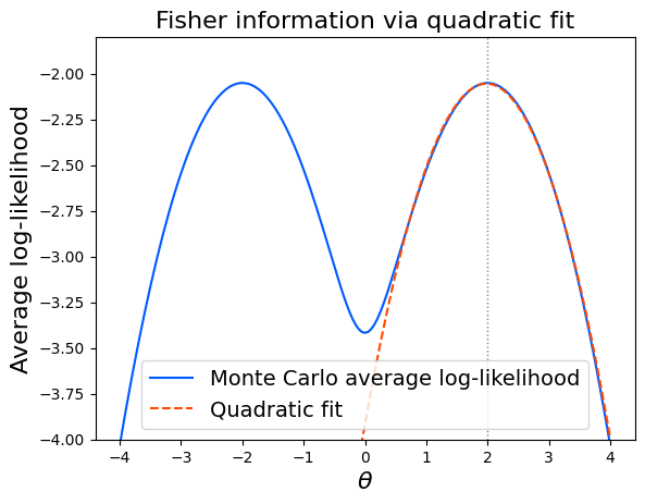
Even though the likelihood is multimodal, a local quadratic fit still provides a usable estimate of the Fisher information.

Fisher Information for Independent and Identically Distributed Data

For independent and identically distributed samples \(X_1,\dots,X_n\),

$$
\begin{aligned}
\mathrm{FisherInformation}(\theta_0)
&\stackrel{\text{def}}{=}
-\mathbb{E}
\left[
\frac{d^2}{d\theta^2}
\log p(X_1,\dots,X_n\mid\theta)
\bigg|_{\theta=\theta_0}
\right] \\
&=
-\mathbb{E}
\left[
\frac{d^2}{d\theta^2}
\sum_{i=1}^n \log p(X_i\mid\theta)
\bigg|_{\theta=\theta_0}
\right] \\
&=
\sum_{i=1}^n
-\mathbb{E}
\left[
\frac{d^2}{d\theta^2}
\log p(X_i\mid\theta)
\bigg|_{\theta=\theta_0}
\right] \\
&=
n\cdot \mathrm{FisherInformation_{single}}(\theta_0).
\end{aligned}
$$

Thus, Fisher information scales linearly with the number of observations.

Cramér–Rao Lower Bound

For any unbiased estimator \(\hat{\theta}\),

$$
\mathrm{Var}(\hat{\theta})
\ge
\frac{1}{\mathrm{FisherInformation}(\theta_0)}.
$$

For i.i.d. data, this becomes

$$
\mathrm{Var}(\hat{\theta})
\ge
\frac{1}{n\cdot \mathrm{FisherInformation_{single}}(\theta_0)}.
$$

Thus, the standard deviation of \(\hat{\theta}\) satisfies

$$
\mathrm{Std}(\hat{\theta})
\ge
\frac{1}{\sqrt{n\cdot \mathrm{FisherInformation_{single}}(\theta_0)}},
$$

which matches the classical \(O(1/\sqrt{n})\) convergence rate, with Fisher information determining the constant. A larger Fisher information yields faster convergence and more accurate estimation.

Multivariate Case

When the parameter is vector-valued \(\boldsymbol{\theta}=(\theta_1,\dots,\theta_d)\), the Fisher information becomes the Fisher information matrix

$$
\mathbf{I}(\boldsymbol{\theta_0})
\stackrel{\text{def}}{=}
-\mathbb{E}_{X\sim p(x\mid\boldsymbol{\theta_0})}
\left[
\nabla_{\boldsymbol{\theta}}^2
\log p(X\mid\boldsymbol{\theta})
\bigg|_{\boldsymbol{\theta}=\boldsymbol{\theta_0}}
\right].
$$

The Cramér–Rao bound generalizes to matrix inequalities involving the covariance matrix and the inverse Fisher information matrix.

Summary

Fisher information is a fundamental quantity describing how precisely model parameters can be estimated.
It can be interpreted as the curvature of the cross-entropy or KL divergence.
For independent and identically distributed data, it increases linearly with the sample size.
The Cramér–Rao inequality shows that a larger Fisher information enables more accurate parameter estimation.

Author Profile

If you found this article useful or interesting, I would be delighted if you could share your thoughts on social media.

New posts are announced on @joisino_en (Twitter), so please be sure to follow!